Fast Fourier Transform

This example shows how to apply a Fast Fourier Transform (FFT) to a pyvista.ImageData using pyvista.ImageDataFilters.fft() filter.

Here, we demonstrate FFT usage by denoising an image, effectively removing any “high frequency” content by performing a low pass filter.

This example was inspired by Image denoising by FFT.

import numpy as np
import pyvista as pv
from pyvista import examples

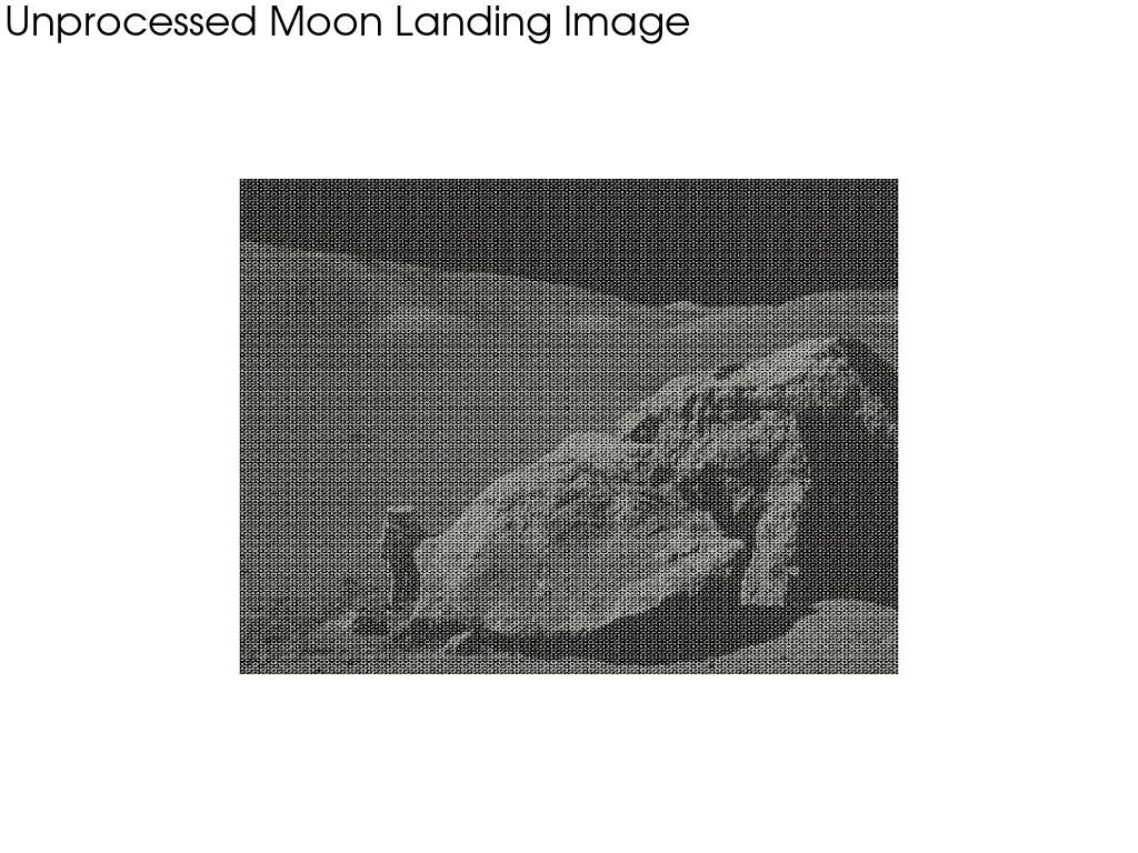
Load the example Moon landing image and plot it.

image = examples.download_moonlanding_image()
print(image.point_data)

# Create a theme that we can reuse when plotting the image
grey_theme = pv.themes.DocumentTheme()
grey_theme.cmap = 'gray'
grey_theme.show_scalar_bar = False
grey_theme.axes.show = False
image.plot(theme=grey_theme, cpos='xy', text='Unprocessed Moon Landing Image')

pyvista DataSetAttributes
Association     : POINT
Active Scalars  : PNGImage
Active Vectors  : None
Active Texture  : None
Active Normals  : None
Contains arrays :
    PNGImage                uint8      (298620,)            SCALARS

Apply FFT to the image

FFT will be applied to the active scalars, 'PNGImage', the default scalars name when loading a PNG image.

The output from the filter is a complex array stored by the same name unless specified using output_scalars_name.

fft_image = image.fft()
fft_image.point_data

pyvista DataSetAttributes
Association     : POINT
Active Scalars  : PNGImage
Active Vectors  : None
Active Texture  : None
Active Normals  : None
Contains arrays :
    PNGImage                complex128 (298620,)            SCALARS

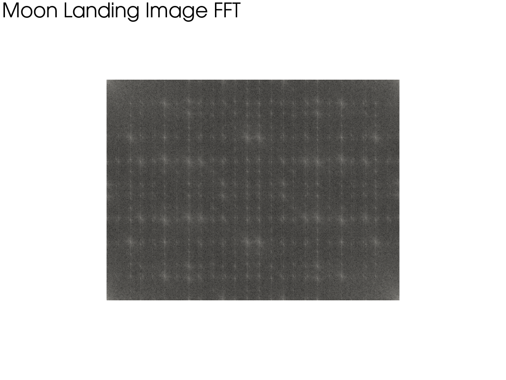
Plot the FFT of the image

Plot the absolute value of the FFT of the image. This is a visualization of the frequency spectrum, not a spatial image — each pixel represents the amplitude of a frequency component, not a location in the moon landing photo.

Note that we are effectively viewing the “frequency” of the data in this image, where the four corners contain the low frequency content of the image, and the middle is the high frequency content of the image.

fft_image.plot(
    scalars=np.abs(fft_image.point_data['PNGImage']),
    cpos='xy',
    theme=grey_theme,
    log_scale=True,
    text='Moon Landing Image FFT Spectrum',
    copy_mesh=True,  # don't overwrite scalars when plotting
)

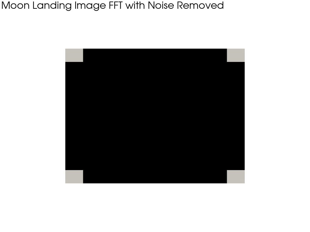
Remove the noise from the fft_image

Effectively, we want to remove high frequency (noisy) data from our image. This is still done in the frequency domain — we are modifying the spectrum, not the spatial image. First, let’s reshape by the size of the image.

Next, perform a low pass filter by removing the middle 80% of the content of the image. Note that the high frequency content is in the middle of the array.

Note

It is easier and more efficient to use the existing pyvista.ImageDataFilters.low_pass() filter. This section is here for demonstration purposes.

ratio_to_keep = 0.10

# modify the fft_image data
width, height, _ = fft_image.dimensions
data = fft_image['PNGImage'].reshape(height, width)  # note: axes flipped
data[int(height * ratio_to_keep) : -int(height * ratio_to_keep)] = 0
data[:, int(width * ratio_to_keep) : -int(width * ratio_to_keep)] = 0

# Set an explicit clim with a positive lower bound; zeroed pixels would
# otherwise break ``log_scale`` (``log10(0) = -inf``) and render as black.
abs_data = np.abs(data)
clim = [abs_data[abs_data > 0].min(), abs_data.max()]

fft_image.plot(
    scalars=abs_data,
    cpos='xy',
    theme=grey_theme,
    log_scale=True,
    clim=clim,
    text='Filtered FFT Spectrum (High Frequencies Zeroed)',
    copy_mesh=True,  # don't overwrite scalars when plotting
)

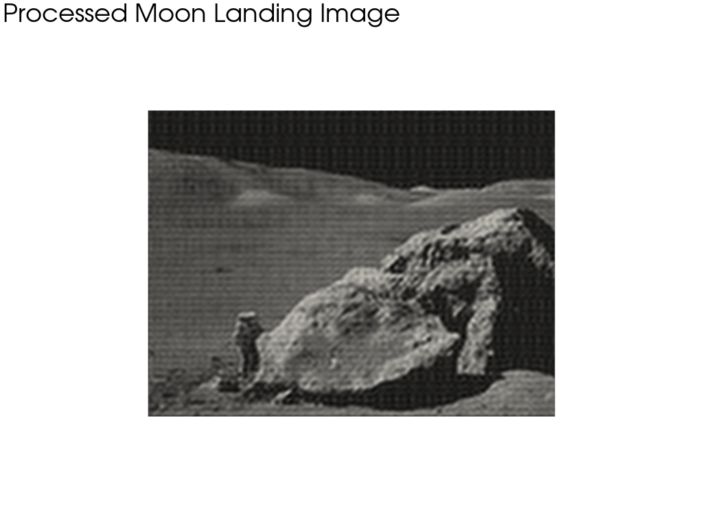
Convert to the spatial domain using reverse FFT

Finally, convert the filtered spectrum back to the spatial domain using the inverse FFT. This is the actual denoised image.

rfft = fft_image.rfft()
rfft['PNGImage'] = np.real(rfft['PNGImage'])
rfft.plot(
    cpos='xy',
    theme=grey_theme,
    text='Denoised Moon Landing Image (Inverse FFT)',
)

Tags: filter