principal_axes#
- principal_axes( ) NumpyArray[float] | tuple[NumpyArray[float], NumpyArray[float]][source]#
Compute the principal axes of a set of points.
Principal axes are orthonormal vectors that best fit a set of points. The axes are also known as the principal components in Principal Component Analysis (PCA), or the right singular vectors from the Singular Value Decomposition (SVD).
The axes are computed as the eigenvectors of the covariance matrix from the mean-centered points, and are processed to ensure that they form a right-handed coordinate frame.
The axes explain the total variance of the points. The first axis explains the largest percentage of variance, followed by the second axis, followed again by the third axis which explains the smallest percentage of variance.
The axes may be used to build an oriented bounding box or to align the points to another set of axes (e.g. the world XYZ axes).
Note
The computed axes are not unique, and the sign of each axis direction can be arbitrarily changed.
Note
This implementation creates a temporary array of the same size as the input array, and is therefore not optimal in terms of its memory requirements. A more memory-efficient computation may be supported in a future release.
Added in version 0.45.0.
- Parameters:
- points
MatrixLike[float] Nx3 array of points.
- return_stdbool, default:
False If
True, also returns the standard deviation of the points along each axis. Standard deviation is computed as the square root of the eigenvalues of the mean-centered covariance matrix.
- points
- Returns:
numpy.ndarray3x3 orthonormal array with the principal axes as row vectors.
numpy.ndarrayThree-item array of the standard deviations along each axis.
See also
fit_plane_to_pointsFit a plane to points using the first two principal axes.
pyvista.DataSetFilters.align_xyzFilter which aligns principal axes to the x-y-z axes.
Examples
>>> import pyvista as pv
>>> import numpy as np
>>> rng = np.random.default_rng(seed=0)  # only seeding for the example
Create a mesh with points that have the largest variation in
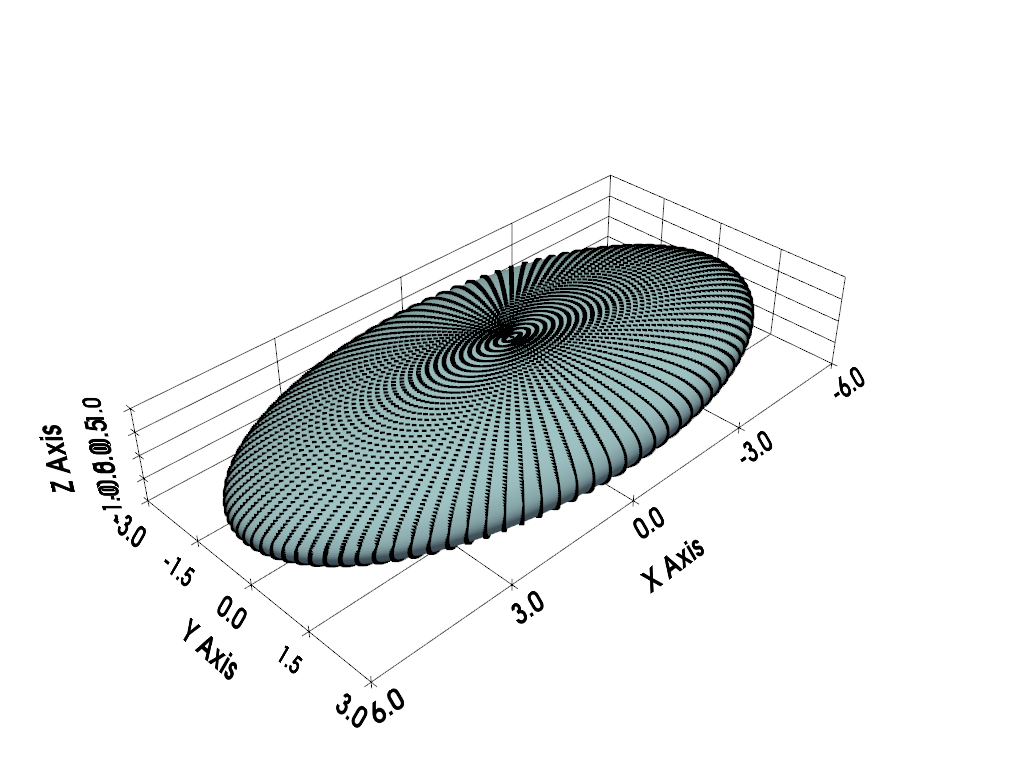
X, followed byY, thenZ.>>> radii = np.array((6, 3, 1)) # x-y-z radii >>> mesh = pv.ParametricEllipsoid( ... xradius=radii[0], yradius=radii[1], zradius=radii[2] ... )
Plot the mesh and highlight its points in black.
>>> pl = pv.Plotter()
>>> _ = pl.add_mesh(mesh)
>>> _ = pl.add_points(mesh, color='black')
>>> _ = pl.show_grid()
>>> pl.show()

Compute its principal axes and return the standard deviations.
>>> axes, std = pv.principal_axes(mesh.points, return_std=True)
>>> axes
pyvista_ndarray([[-1.,  0.,  0.],
                 [ 0.,  1.,  0.],
                 [ 0.,  0., -1.]], dtype=float32)
Note that the principal axes have ones along the diagonal and zeros in the off-diagonal. This indicates that the first principal axis is aligned with the x-axis, the second with the y-axis, and third with the z-axis. This is expected, since the mesh is already axis-aligned.
However, since the signs of the principal axes are arbitrary, the first and third axes in this case have a negative direction.
Show the standard deviation along each axis.
>>> std
array([3.0149 , 1.5074 , 0.7035], dtype=float32)
Compare this to using
numpy.std()for the computation.>>> np.std(mesh.points, axis=0) pyvista_ndarray([3.0149572, 1.5074761, 0.7035699], dtype=float32)
Since the points are axis-aligned, the two results agree in this case. In general, however, these two methods differ in that
numpy.std()with axis=0 computes the standard deviation along the x-y-z axes, whereas the standard deviation returned byprincipal_axes()is computed along the principal axes.Convert the values to proportions for analysis.
>>> std / sum(std)
array([0.5769149 , 0.28845742, 0.1346276 ], dtype=float32)
From this result, we can determine that the axes explain approximately 58%, 29%, and 13% of the total variance in the points, respectively.
Let’s compare this to the proportions of the known radii of the ellipsoid.
>>> radii / sum(radii)
array([0.6, 0.3, 0.1])
Note how the two ratios are similar, but do not match exactly. This is because the points of the ellipsoid are prolate and are denser near the poles. If the points were normally distributed, however, the proportions would match exactly.
Create an array of normally distributed points scaled along the x-y-z axes. Use the same scaling as the radii of the ellipsoid from the previous example.
>>> normal_points = rng.normal(size=(1000, 3))
>>> scaled_points = normal_points * radii
>>> axes, std = pv.principal_axes(scaled_points, return_std=True)
>>> axes
array([[-0.99997578,  0.00682346,  0.00136972],
       [ 0.00681368,  0.99995213, -0.00702282],
       [-0.00141757, -0.00701331, -0.9999744 ]])
Once again, the axes have ones along the diagonal as expected since the points are already axis-aligned. Now let’s examine the standard deviation and compare the relative proportions.
>>> std
array([5.94466738, 2.89590334, 1.02103169])
>>> std / sum(std)
array([0.60280948, 0.29365444, 0.10353608])
>>> radii / sum(radii)
array([0.6, 0.3, 0.1])
Since the points are normally distributed, the relative proportion of the standard deviation matches the scaling of the axes almost perfectly.