Note
Go to the end to download the full example code.
Compare interpolation/sampling methods#
There are two main methods of interpolating or sampling data from a target mesh
in PyVista. pyvista.DataSetFilters.interpolate() uses a distance weighting
kernel to interpolate point data from nearby points of the target mesh onto
the desired points.
pyvista.DataObjectFilters.sample() interpolates data using the
interpolation scheme of the enclosing cell from the target mesh.
If the target mesh is a point cloud, i.e. there is no connectivity in the cell
structure, then pyvista.DataSetFilters.interpolate() is typically
preferred. If interpolation is desired within the cells of the target mesh, then
pyvista.DataObjectFilters.sample() is typically desired.
Here the two methods are compared and contrasted using a simple example of sampling data from a mesh in a rectangular domain. This example demonstrates the main differences above. For more complex uses, see Detailed Interpolating Points and Detailed Resampling.
import numpy as np
import pyvista as pv
Interpolating from point cloud#
A point cloud is a collection of points that have no connectivity in
the mesh, i.e. the mesh contains no cells or the cells are 0D
(vertex or polyvertex). The filter pyvista.DataSetFilters.interpolate()
uses a distance-based weighting methodology to interpolate between the
unconnected points.
First, generate a point cloud mesh in a rectangular domain from
(0, 0) to (3, 1). The data to be sampled is the square of the y position.
rng = np.random.default_rng(seed=0)
points = rng.uniform(low=[0, 0], high=[3, 1], size=(250, 2))
# Make points be z=0
points = np.hstack((points, np.zeros((250, 1))))
point_mesh = pv.PolyData(points)
point_mesh['ysquared'] = points[:, 1] ** 2
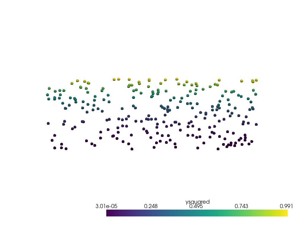
The point cloud data looks like this.
pl = pv.Plotter()
pl.add_mesh(point_mesh, render_points_as_spheres=True, point_size=10)
pl.view_xy()
pl.show()

Now estimate data on a regular grid from the point data. Note
that the distance parameter radius determines how far away to
look for point cloud data.
grid = pv.ImageData(dimensions=(11, 11, 1), spacing=[3 / 10, 1 / 10, 1])
output = grid.interpolate(point_mesh, radius=0.1, null_value=-1)
output
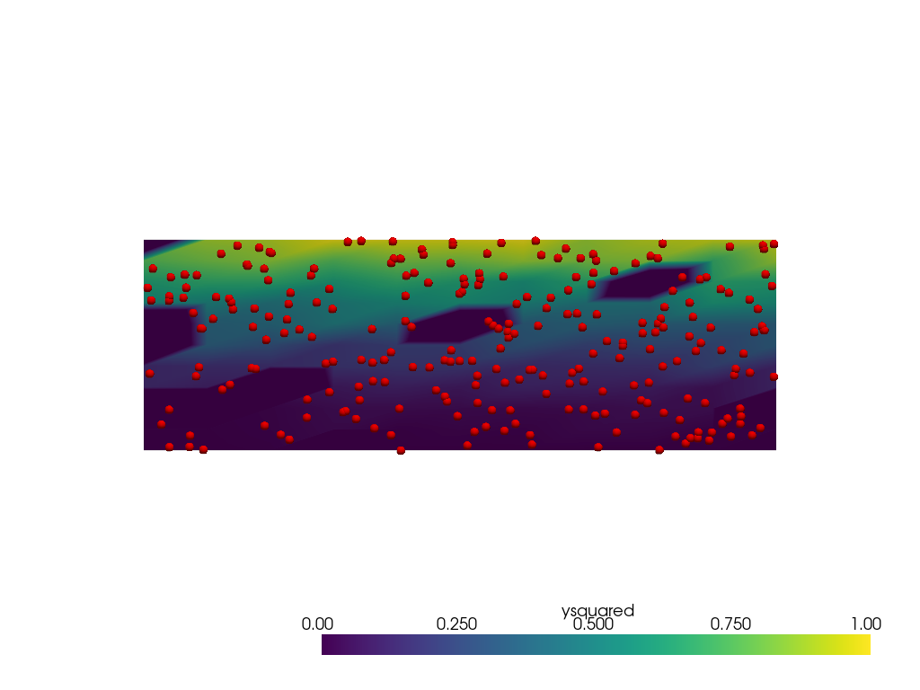
When using radius=0.1, the expected extents of the data are
captured reasonably well over the domain, but there are holes in the
data (represented by the darkest blue colors) caused by no points within
the radius to interpolate from.
pl = pv.Plotter()
pl.add_mesh(output, clim=[0, 1])
pl.add_mesh(points, render_points_as_spheres=True, point_size=10, color='red')
pl.view_xy()
pl.show()
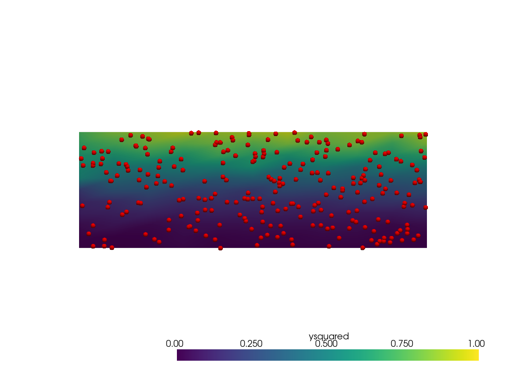
Now repeat with radius=0.25.
There are no holes but the extents of the data is much narrower
than [0, 1]. This is caused by more interior points involved
in the weighting near the lower and upper edges of the domain.
Other parameters such as sharpness could be tuned to try to
lessen the issue.
grid = pv.ImageData(dimensions=(11, 11, 1), spacing=[3 / 10, 1 / 10, 1])
output = grid.interpolate(point_mesh, radius=0.25, null_value=-1)

pl = pv.Plotter()
pl.add_mesh(output, clim=[0, 1])
pl.add_mesh(points, render_points_as_spheres=True, point_size=10, color='red')
pl.view_xy()
pl.show()
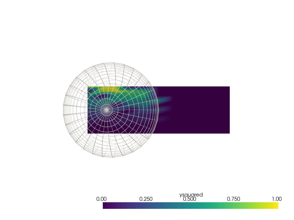
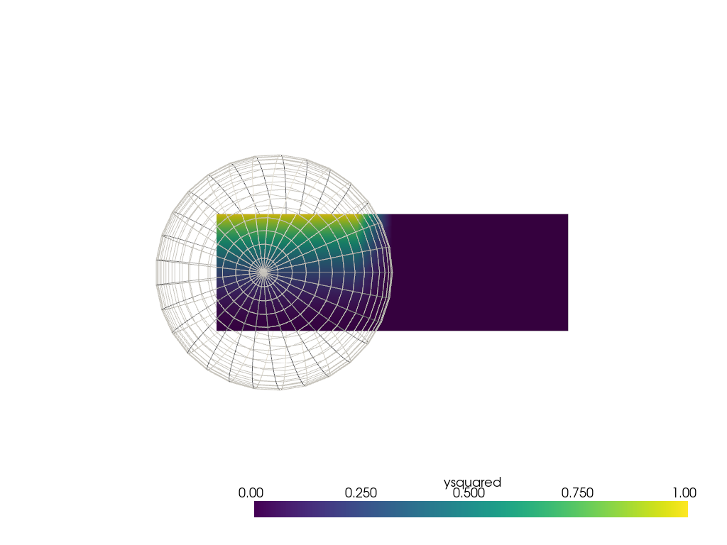
While this filter is very useful for point clouds, it is possible to use
it to interpolate from the points on other mesh types. With
an unsuitable choice of radius the interpolation doesn’t look very good.
It is recommended consider using pyvista.DataObjectFilters.sample() in a
case like this (see next section below). However, there may be cases with
non-point cloud meshes where pyvista.DataSetFilters.interpolate() is
still preferred.
sphere = pv.SolidSphere(center=(0.5, 0.5, 0), outer_radius=1.0)
sphere['ysquared'] = sphere.points[:, 1] ** 2
output = grid.interpolate(sphere, radius=0.1)

pl = pv.Plotter()
pl.add_mesh(output, clim=[0, 1])
pl.add_mesh(sphere, style='wireframe', color='white')
pl.view_xy()
pl.show()
Sampling from a mesh with connectivity#
This example is in many ways the opposite of the prior one.
A mesh with cell connectivity that spans 2 dimensions is
sampled at discrete points using pyvista.DataObjectFilters.sample().
Importantly, the cell connectivity enables direct interpolation
inside the domain without needing distance or weighting parametization.
First, show that sample does not work with point clouds with data.
Either pyvista.DataSetFilters.interpolate() or the
snap_to_closest_point parameter must be used.
grid = pv.ImageData(dimensions=(11, 11, 1), spacing=[3 / 10, 1 / 10, 1])
output = grid.sample(point_mesh)
# value of (0, 0) shows that no data was sampled
print(f'(min, max): {output["ysquared"].min()}, {output["ysquared"].min()}')
(min, max): 0.0, 0.0
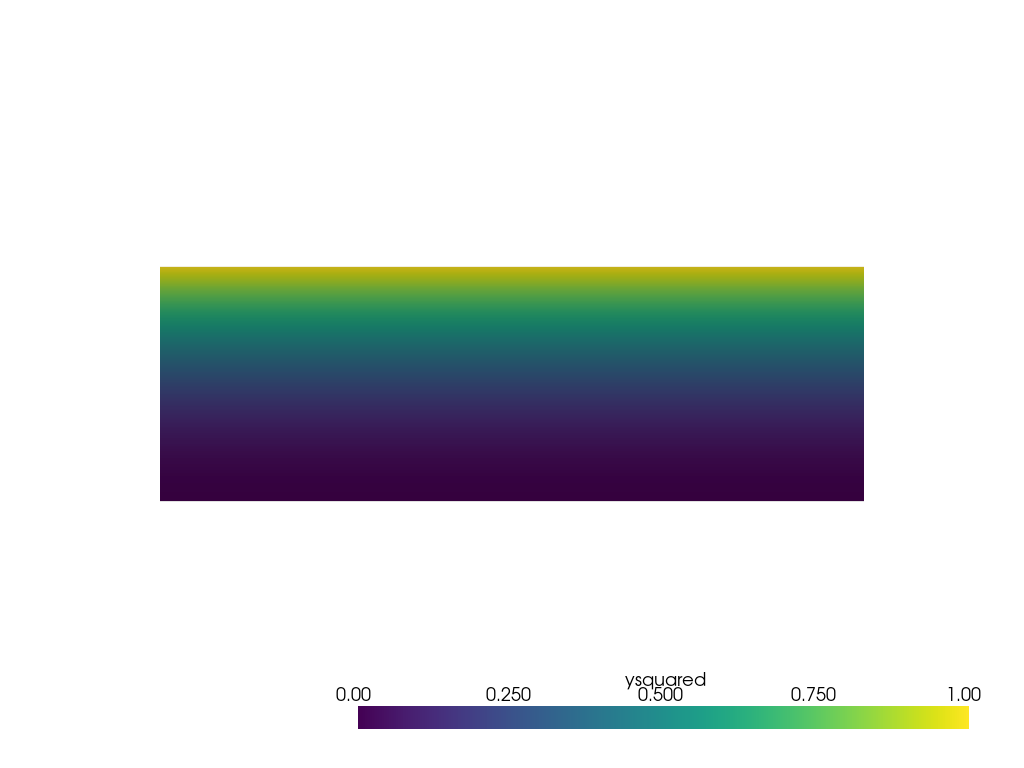
Create the non-point cloud mesh that will be sampled from and plot it.
grid = pv.ImageData(dimensions=(11, 11, 1), spacing=[3 / 10, 1 / 10, 1])
grid['ysquared'] = grid.points[:, 1] ** 2

pl = pv.Plotter()
pl.add_mesh(grid, clim=[0, 1])
pl.view_xy()
pl.show()
Now sample it at the discrete points used in the first example.
This looks identical to the first plot of the first example as the data is not noisy, and there is little interpolation error.
pl = pv.Plotter()
pl.add_mesh(output, render_points_as_spheres=True, point_size=10)
pl.view_xy()
pl.show()
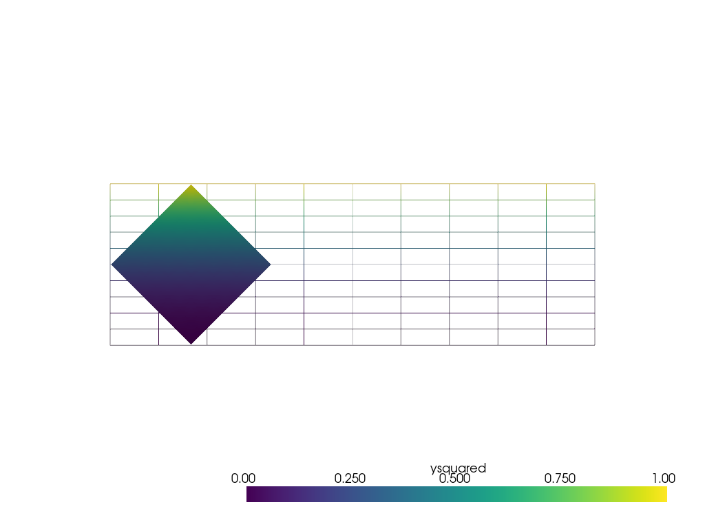
Instead of sampling onto a point cloud, pyvista.DataObjectFilters.sample()
can sample using other mesh types. For example, sampling onto a rotated subset
of the grid.
Make subset (0.7, 0.7, 0) units in dimension and then rotate by 45 degrees around its center.
subset = pv.ImageData(dimensions=(8, 8, 1), spacing=[0.1, 0.1, 0], origin=(0.15, 0.15, 0))
rotated_subset = subset.rotate_vector(vector=(0, 0, 1), angle=45, point=(0.5, 0.5, 0))
output = rotated_subset.sample(grid)
output
The data in the sampled region looks identical to the original grid due to the well-behaved nature of the data and low interpolation error.
pl = pv.Plotter()
pl.add_mesh(grid, style='wireframe', clim=[0, 1])
pl.add_mesh(output, clim=[0, 1])
pl.view_xy()
pl.show()
Repeat the sphere interpolation example, but using
pyvista.DataObjectFilters.sample(). This method
is directly able to sample from the mesh in this case without
fiddling with distance weighting parameters.
sphere = pv.SolidSphere(center=(0.5, 0.5, 0), outer_radius=1.0)
sphere['ysquared'] = sphere.points[:, 1] ** 2
output = grid.sample(sphere)

pl = pv.Plotter()
pl.add_mesh(output, clim=[0, 1])
pl.add_mesh(sphere, style='wireframe', color='white')
pl.view_xy()
pl.show()
Total running time of the script: (0 minutes 2.268 seconds)