Note
Go to the end to download the full example code.
Creating a Spline#
Create a spline/polyline from a numpy array of XYZ vertices using
pyvista.Spline().
import numpy as np

import pyvista as pv
Create a dataset to plot
def make_points():
    """Make XYZ points."""
    theta = np.linspace(-4 * np.pi, 4 * np.pi, 100)
    z = np.linspace(-2, 2, 100)
    r = z**2 + 1
    x = r * np.sin(theta)
    y = r * np.cos(theta)
    return np.column_stack((x, y, z))


points = make_points()
points[0:5, :]
array([[ 2.44929360e-15,  5.00000000e+00, -2.00000000e+00],
       [ 1.21556036e+00,  4.68488752e+00, -1.95959596e+00],
       [ 2.27700402e+00,  4.09249671e+00, -1.91919192e+00],
       [ 3.12595020e+00,  3.27840221e+00, -1.87878788e+00],
       [ 3.72150434e+00,  2.30906573e+00, -1.83838384e+00]])
Now let’s make a function that can create line cells on a
pyvista.PolyData mesh given that the points are in order for the
segments they make.
def lines_from_points(points):
    """Given an array of points, make a line set."""
    poly = pv.PolyData()
    poly.points = points
    cells = np.full((len(points) - 1, 3), 2, dtype=np.int_)
    cells[:, 1] = np.arange(0, len(points) - 1, dtype=np.int_)
    cells[:, 2] = np.arange(1, len(points), dtype=np.int_)
    poly.lines = cells
    return poly


line = lines_from_points(points)
line
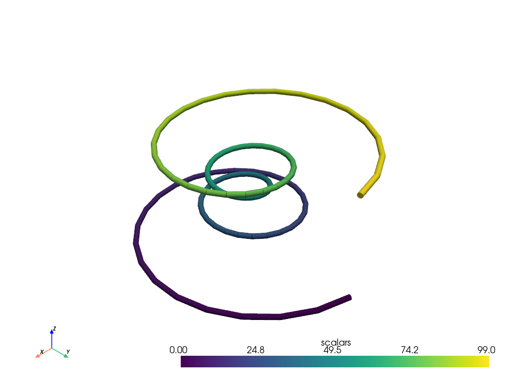
That tube has sharp edges at each line segment. This can be mitigated by creating a single PolyLine cell for all of the points
def polyline_from_points(points):
    poly = pv.PolyData()
    poly.points = points
    the_cell = np.arange(0, len(points), dtype=np.int_)
    the_cell = np.insert(the_cell, 0, len(points))
    poly.lines = the_cell
    return poly


polyline = polyline_from_points(points)
polyline['scalars'] = np.arange(polyline.n_points)
tube = polyline.tube(radius=0.1)
tube.plot(smooth_shading=True)

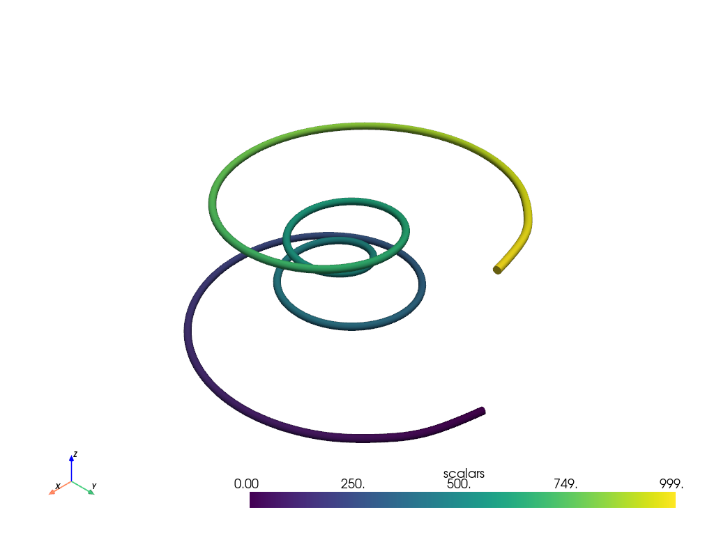
You could also interpolate those points onto a parametric spline
Plot spline as a tube
# add scalars to spline and plot it
spline['scalars'] = np.arange(spline.n_points)
tube = spline.tube(radius=0.1)
tube.plot(smooth_shading=True)
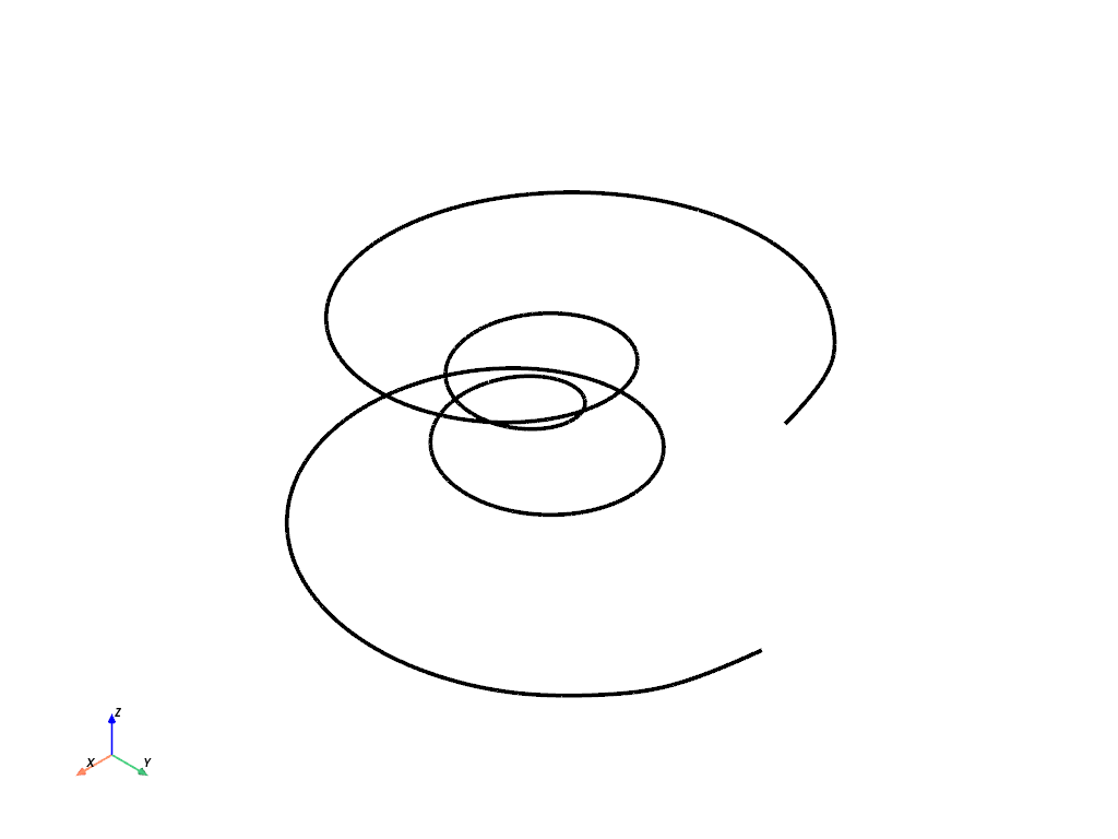
The spline can also be plotted as a plain line
# generate same spline with 400 interpolation points
spline = pv.Spline(points, 400)

# plot without scalars
spline.plot(line_width=4, color='k')
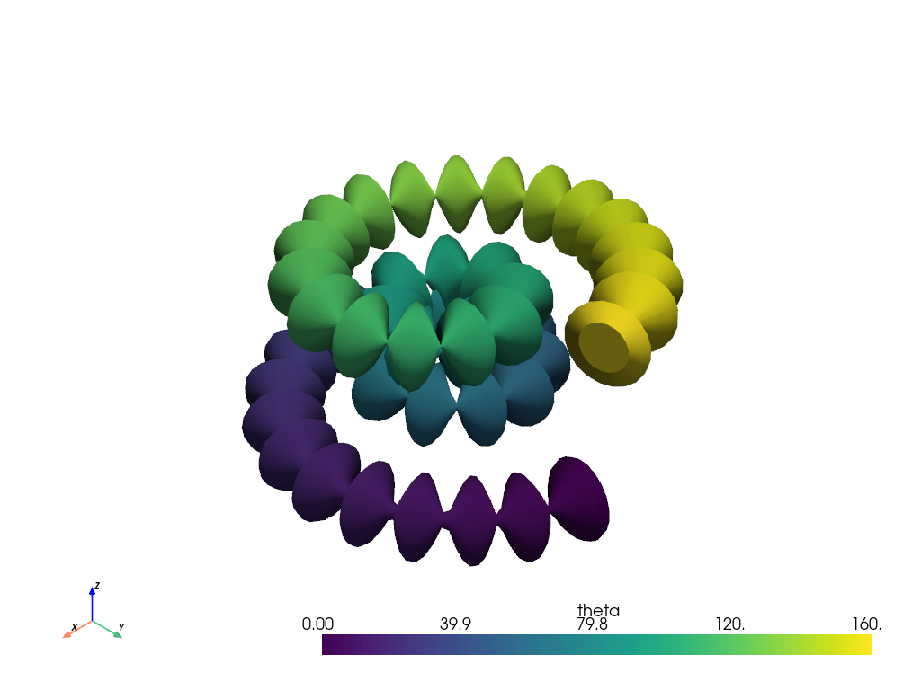
The radius of the tube can be modulated with scalars
spline['theta'] = 0.4 * np.arange(len(spline.points))
spline['radius'] = np.abs(np.sin(spline['theta']))
tube = spline.tube(scalars='radius', absolute=True)
tube.plot(scalars='theta', smooth_shading=True)
Ribbons#
Any of the lines from the examples above can be used to create ribbons.
Take a look at the pyvista.PolyDataFilters.ribbon() filter.
ribbon = spline.compute_arc_length().ribbon(width=0.75, scalars='arc_length')
ribbon.plot(color=True)

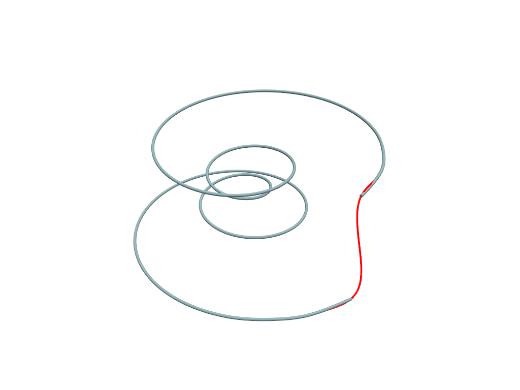
Closing a Spline#
Create a spline and its closed counterpart.
spline = pv.Spline(points, 1000)
spline_closed = pv.Spline(points, 1000, closed=True)
pl = pv.Plotter()
pl.add_mesh(spline.tube(radius=0.05))
pl.add_mesh(spline_closed, line_width=4, color='r')
pl.show()
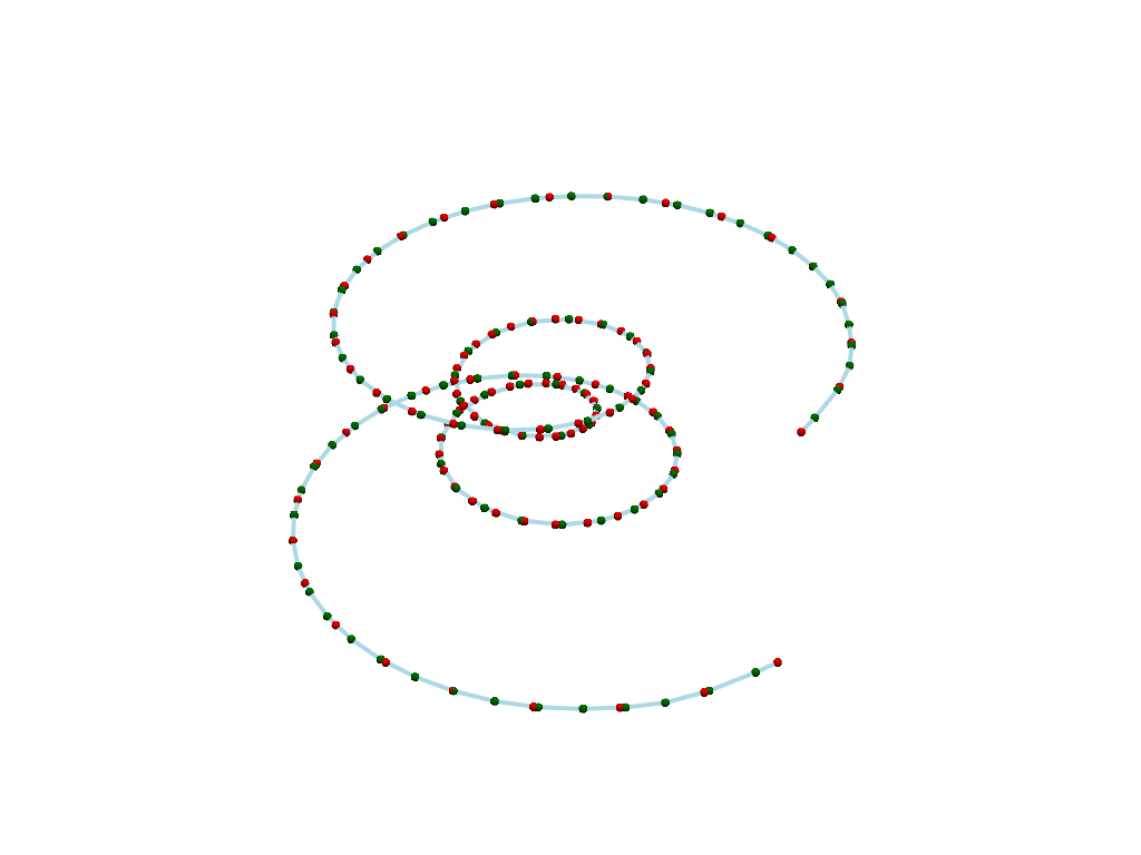
Parametrizing by Length Versus Index#
Create a spline by parametrizing based on length (default) or point index.
pl = pv.Plotter()
spline = pv.Spline(points, parametrize_by='length')
spline_by_index = pv.Spline(points, parametrize_by='index')
pl.add_mesh(spline, line_width=4)
pl.add_mesh(spline.points, color='g', point_size=8.0, render_points_as_spheres=True)
pl.add_mesh(
    spline_by_index.points, color='r', point_size=8.0, render_points_as_spheres=True
)
pl.show()
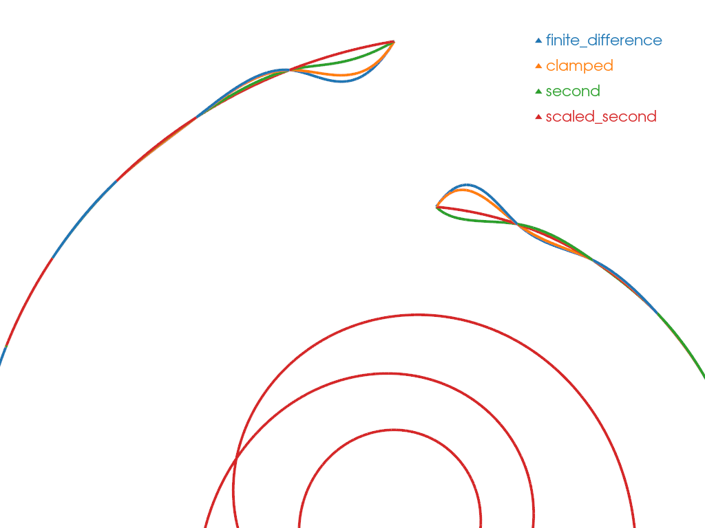
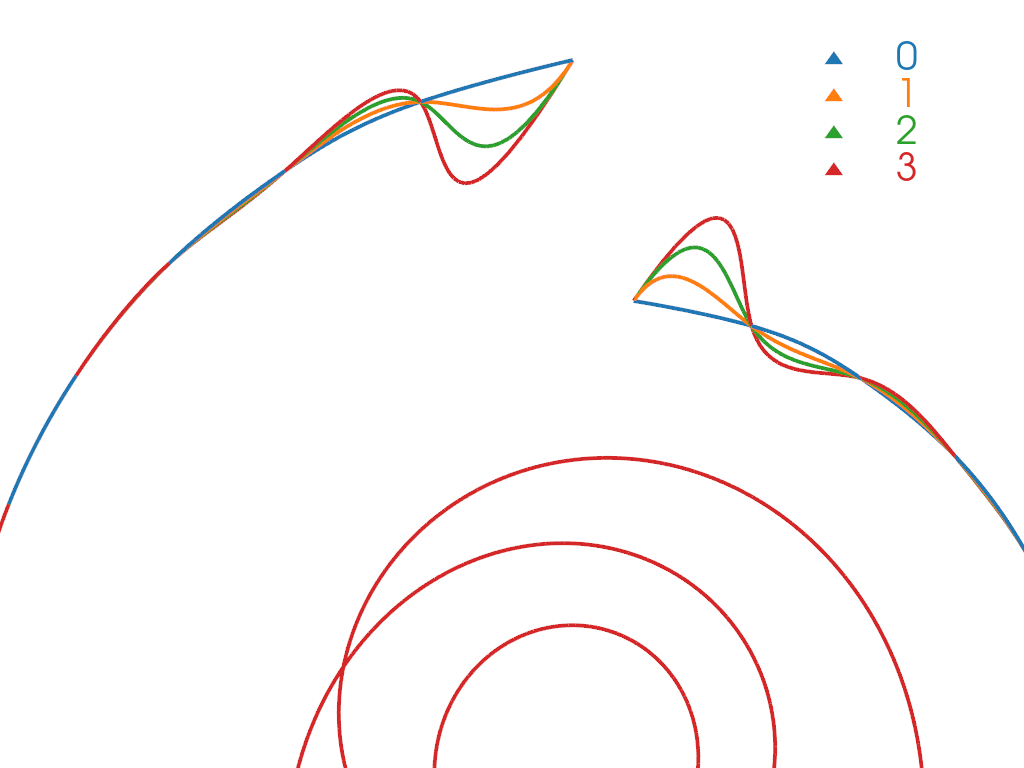
Boundary Constraints#
Create a spline and see the effect of boundary constraint.
Boundary type can be ‘finite_difference’, ‘clamped’, ‘second’, ‘scaled_second’
with the definition of the boundary types in pyvista.Spline().
To visualize the different splines, we label each one using integer ID scalars and merge them into a single mesh.
pl = pv.Plotter()
mesh = pv.PolyData()
constraint_map = {'finite_difference': 0, 'clamped': 1, 'second': 2, 'scaled_second': 3}
for constraint, constraint_id in constraint_map.items():
    val = None if constraint == 'finite_difference' else 1.0
    spline = pv.Spline(
        points,
        1000,
        boundary_constraints=constraint,
        boundary_values=val,
    )
    spline.cell_data['boundary_constraint'] = np.array([constraint_id], dtype=np.uint8)
    mesh = pv.merge([mesh, spline], merge_points=False)

colored_mesh, color_map = mesh.color_labels(
    output_scalars='boundary_constraint', return_dict=True
)
legend_map = dict(zip(constraint_map.keys(), color_map.values(), strict=True))
pl.add_mesh(colored_mesh, line_width=4, rgb=True)
pl.add_legend(legend_map)
cpos = pv.CameraPosition(
    position=(2.0, -2.0, 11.0), focal_point=(-0.8, 3.3, -0.4), viewup=(0.0, 1.0, 0.5)
)
pl.camera_position = cpos
pl.show()
Boundary Values#
Create a spline and see the effect of boundary value. It can be set at left and right value and has no effect for boundary type 0.
pl = pv.Plotter()
mesh = pv.PolyData()
for boundary_value in range(4):
    spline = pv.Spline(
        points,
        1000,
        boundary_constraints='clamped',
        boundary_values=boundary_value,
    )
    spline.cell_data['boundary_value'] = np.array([boundary_value], dtype=float)
    mesh = pv.merge([mesh, spline], merge_points=False)

colored_mesh, color_map = mesh.color_labels(
    output_scalars='boundary_value', return_dict=True
)
pl.add_mesh(colored_mesh, line_width=4, rgb=True)
pl.add_legend(color_map)
pl.camera_position = cpos
pl.show()
Total running time of the script: (0 minutes 2.441 seconds)