Maximum Intensity Projection

Maximum Intensity Projection (MIP) is a rendering technique for point clouds that reorders vertex depth so points with higher scalar values are always rendered in front, regardless of their actual distance from the camera.

This is useful for dense point cloud visualization where high-value data points would otherwise be hidden behind lower-value points that happen to be closer to the viewer. The technique was proposed by Cowan (2014) for visualizing grade data in mining applications, where it is referred to as “X-ray plunge projection.”

MIP works by replacing the z-coordinate in OpenGL clip space with the negated, normalized scalar value via a custom vertex shader. This means that depth ordering is driven entirely by scalar magnitude rather than spatial position.

import numpy as np
import pyvista as pv
from pyvista import examples

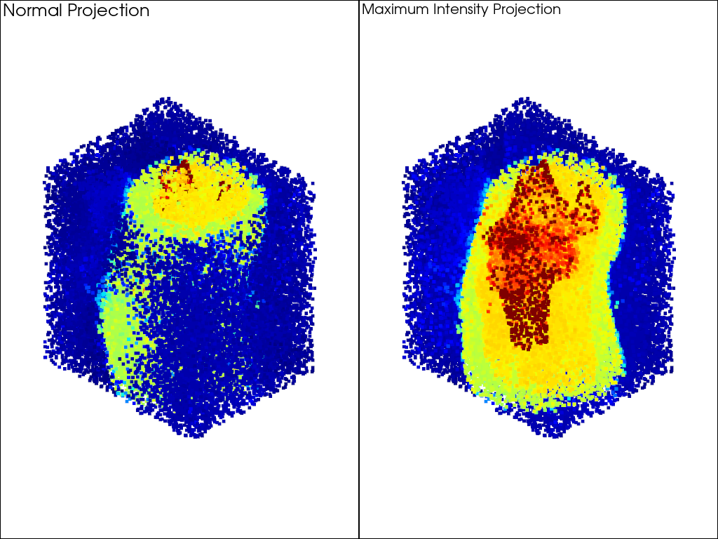
Normal vs. MIP Rendering

Using a sample of the knee dataset, we compare normal rendering (left) where closer points occlude farther ones, with MIP rendering (right) where the highest scalar values punch through to the front.

vol = examples.download_knee_full()

sample_n = 50000
rng = np.random.default_rng(0)
indices = rng.integers(0, vol.n_points, sample_n)
pts = vol.extract_points(indices, adjacent_cells=False, include_cells=False)

display = dict(
    cmap='jet', clim=[0, 100], style='points', point_size=5, show_scalar_bar=False
)

pl = pv.Plotter(shape=(1, 2))
pl.enable_parallel_projection()

pl.subplot(0, 0)
pl.add_mesh(pts, **display)
pl.add_text('Normal Projection', font_size=12)

pl.subplot(0, 1)
mip_actor = pl.add_mesh(pts, **display)
mip_actor.enable_maximum_intensity_projection()
pl.add_text('Maximum Intensity Projection', font_size=12)

pl.link_views()
pl.show()

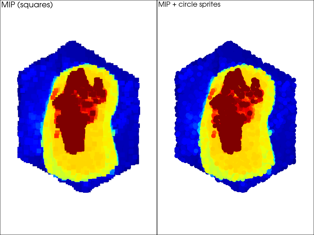
MIP with Circle Point Sprites

MIP modifies the vertex shader while point sprites modify the fragment shader, so both features compose cleanly on the same actor. Using circle sprites with MIP produces a cleaner visualization than the default square points.

combined_display = dict(
    cmap='jet', clim=[0, 100], style='points', point_size=15, show_scalar_bar=False
)

pl = pv.Plotter(shape=(1, 2))
pl.enable_parallel_projection()

pl.subplot(0, 0)
actor_squares = pl.add_mesh(
    pts,
    render_points_as_spheres=False,
    **combined_display,
)
actor_squares.enable_maximum_intensity_projection()
pl.add_text('MIP (squares)', font_size=12)

pl.subplot(0, 1)
actor_circles = pl.add_mesh(
    pts,
    point_shape='circle',
    **combined_display,
)
actor_circles.enable_maximum_intensity_projection()
pl.add_text('MIP + circle sprites', font_size=12)

pl.link_views()
pl.show()

Note

MIP requires VTK >= 9.3.

Note

MIP does not work correctly with opacity < 1 unless depth peeling is enabled. See pyvista.Plotter.enable_depth_peeling().

References

Cowan, E.J., 2014. ‘X-ray Plunge Projection’, Understanding Structural Geology from Grade Data. AusIMM Monograph 30, 207-220.