Point Sets

Point sets are datasets with explicit geometry where the point and cell topology are specified and not inferred.

PolyData

Surface geometry: vertices, lines, polygons, and triangles. Extension of vtkPolyData.

PolyData

UnstructuredGrid

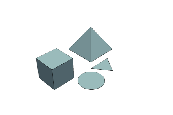
Arbitrary combinations of all cell types for volumetric and surface data. Extension of vtkUnstructuredGrid.

UnstructuredGrid

StructuredGrid

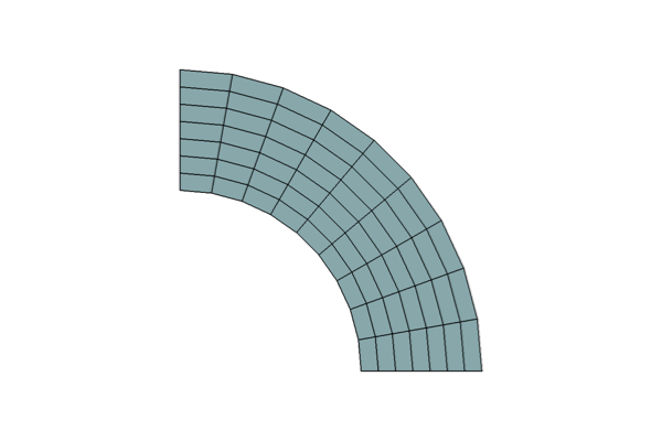
Regular lattice of points with connectivity defined by grid ordering. Extension of vtkStructuredGrid.

StructuredGrid

PointSet

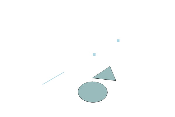
A concrete class for storing a set of points with no cell connectivity. Extension of vtkPointSet.

PointSet

Class Reference

PointSet(*args, **kwargs)	Concrete class for storing a set of points.
PolyData(*args, **kwargs)	Dataset consisting of surface geometry (e.g. vertices, lines, and polygons).
UnstructuredGrid(*args, **kwargs)	Dataset used for arbitrary combinations of all possible cell types.
StructuredGrid(*args, **kwargs)	Dataset used for topologically regular arrays of data.
ExplicitStructuredGrid(*args, **kwargs)	Extend the functionality of the vtkExplicitStructuredGrid class.