Fast Fourier Transform with Perlin Noise

This example shows how to apply a Fast Fourier Transform (FFT) to a pyvista.ImageData using pyvista.ImageDataFilters.fft() filter.

Here, we demonstrate FFT usage by first generating Perlin noise using pyvista.sample_function() to sample pyvista.perlin_noise, and then performing FFT of the sampled noise to show the frequency content of that noise.

import numpy as np

import pyvista as pv

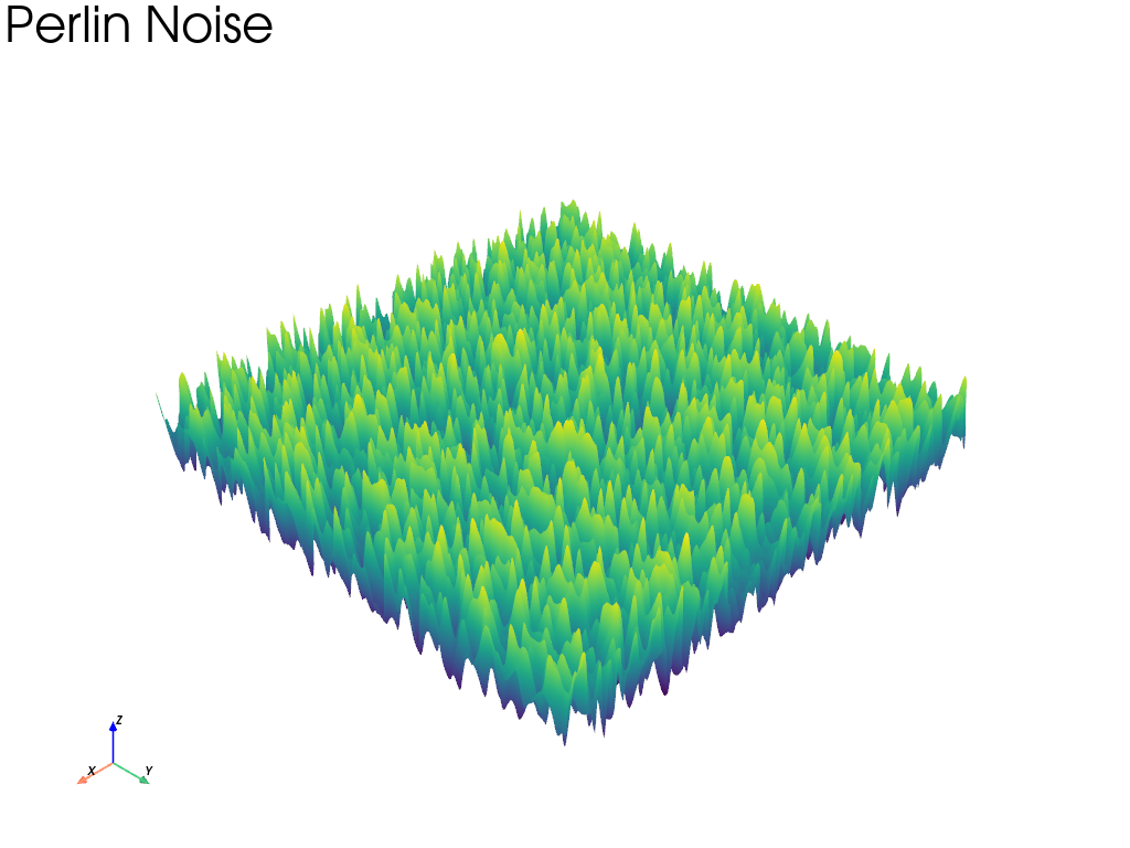
Generate Perlin Noise

Start by generating some Perlin Noise as in Sample Function: Perlin Noise in 2D example.

Note that we are generating it in a flat plane and using a frequency of 10 in the x direction and 5 in the y direction. The unit of frequency is 1/pixel.

Also note that the dimensions of the image are powers of 2. This is because the FFT is much more efficient for arrays sized as a power of 2.

freq = [10, 5, 0]
noise = pv.perlin_noise(1, freq, (0, 0, 0))
xdim, ydim = (2**9, 2**9)
sampled = pv.sample_function(noise, bounds=(0, 10, 0, 10, 0, 10), dim=(xdim, ydim, 1))

# warp and plot the sampled noise
warped_noise = sampled.warp_by_scalar()
warped_noise.plot(show_scalar_bar=False, text='Perlin Noise', lighting=False)

Static Scene

Interactive Scene

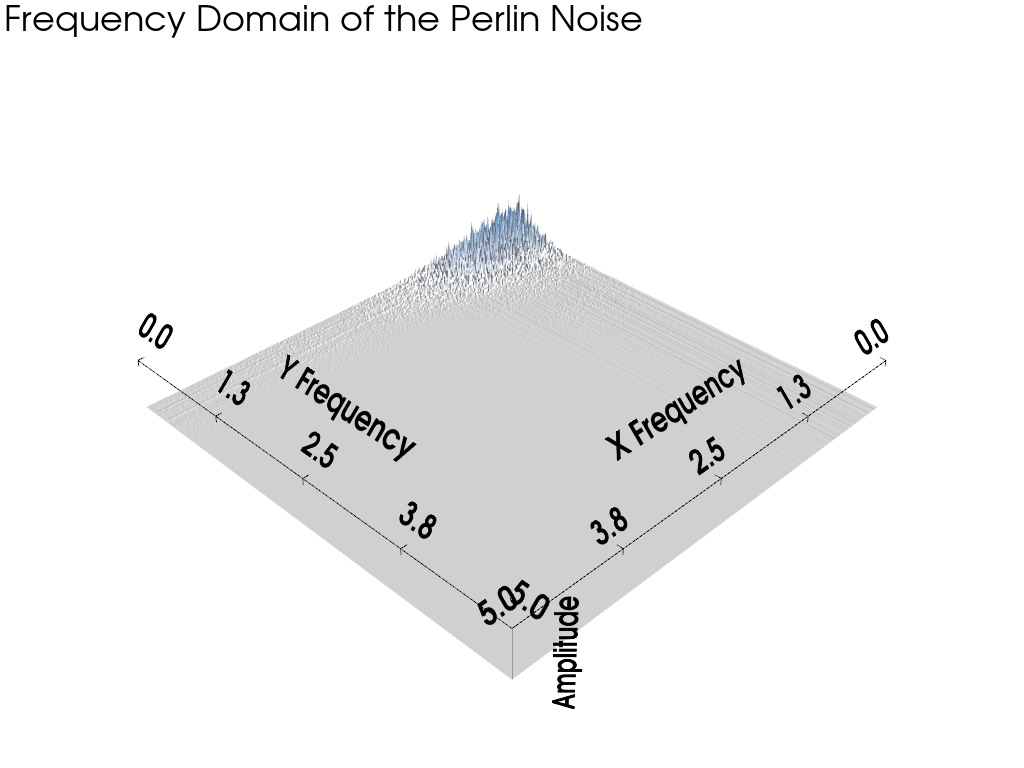
Perform FFT of Perlin Noise

Next, perform an FFT of the noise and plot the frequency content. For the sake of simplicity, we will only plot the content in the first quadrant.

Note the usage of numpy.fft.fftfreq() to get the frequencies.

sampled_fft = sampled.fft()
freq = np.fft.fftfreq(sampled.dimensions[0], sampled.spacing[0])
max_freq = freq.max()

# only show the first quadrant
subset = sampled_fft.extract_subset((0, xdim // 2, 0, ydim // 2, 0, 0))

Plot the Frequency Domain

Now, plot the noise in the frequency domain. Note how there is more high frequency content in the x direction and this matches the frequencies given to pyvista.perlin_noise.

# scale to make the plot viewable
subset['scalars'] = np.abs(subset.active_scalars)
warped_subset = subset.warp_by_scalar(factor=0.0001)

pl = pv.Plotter(lighting='three lights')
pl.add_mesh(warped_subset, cmap='blues', show_scalar_bar=False)
pl.show_bounds(
    axes_ranges=(0, max_freq, 0, max_freq, 0, warped_subset.bounds[-1]),
    xtitle='X Frequency',
    ytitle='Y Frequency',
    ztitle='Amplitude',
    show_zlabels=False,
    color='k',
    font_size=26,
)
pl.add_text('Frequency Domain of the Perlin Noise')
pl.show()

Static Scene

Interactive Scene

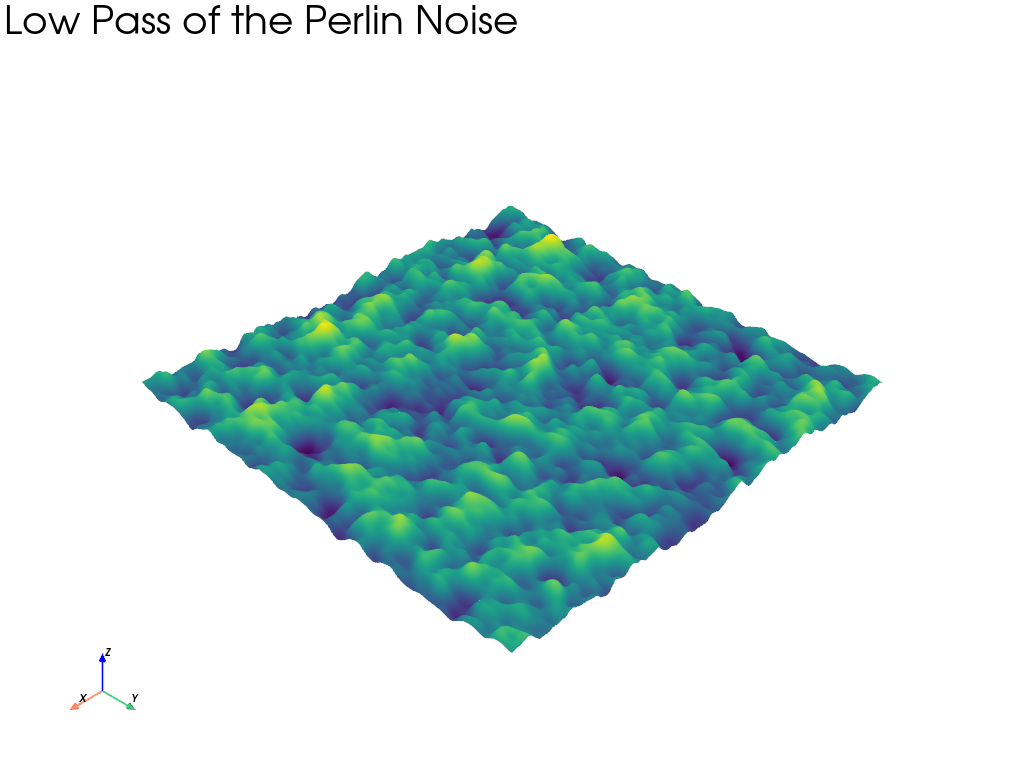
Low Pass Filter

Let’s perform a low pass filter on the frequency content and then convert it back into the space (pixel) domain by immediately applying a reverse FFT.

When converting back, keep only the real content. The imaginary content has no physical meaning in the physical domain. PyVista will drop the imaginary content, but will warn you of it.

As expected, we only see low frequency noise.

low_pass = sampled_fft.low_pass(1.0, 1.0, 1.0).rfft()
low_pass['scalars'] = np.real(low_pass.active_scalars)
warped_low_pass = low_pass.warp_by_scalar()
warped_low_pass.plot(show_scalar_bar=False, text='Low Pass of the Perlin Noise', lighting=False)

Static Scene

Interactive Scene

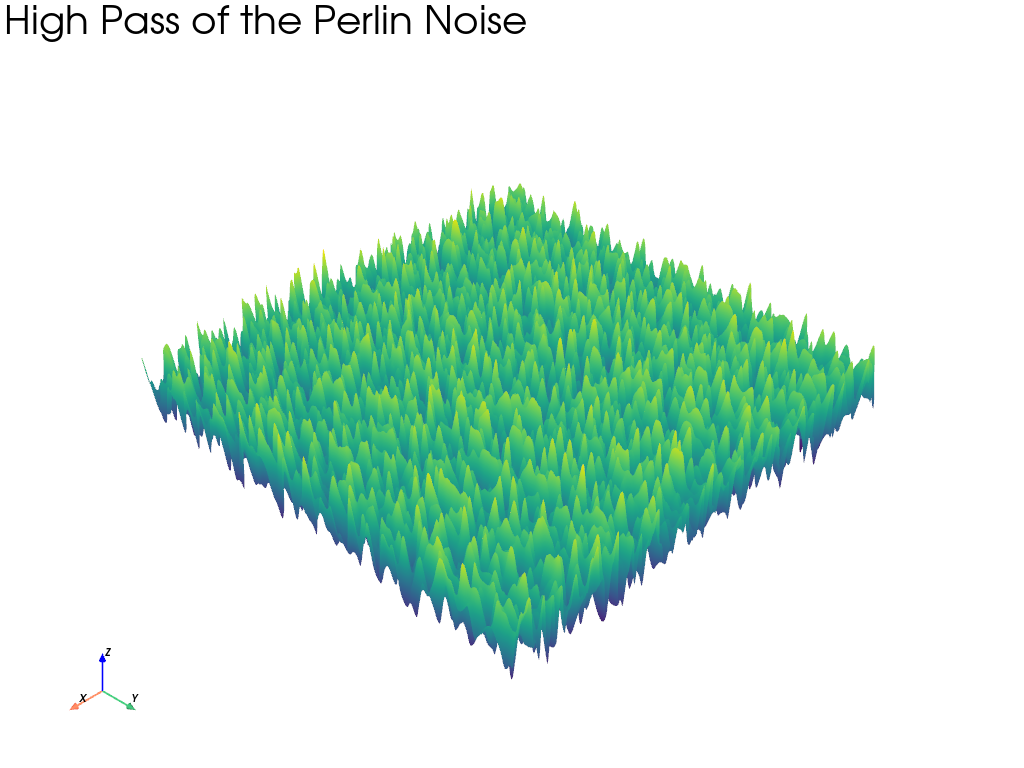
High Pass Filter

This time, let’s perform a high pass filter on the frequency content and then convert it back into the space (pixel) domain by immediately applying a reverse FFT.

When converting back, keep only the real content. The imaginary content has no physical meaning in the pixel domain.

As expected, we only see the high frequency noise content as the low frequency noise has been attenuated.

high_pass = sampled_fft.high_pass(1.0, 1.0, 1.0).rfft()
high_pass['scalars'] = np.real(high_pass.active_scalars)
warped_high_pass = high_pass.warp_by_scalar()
warped_high_pass.plot(show_scalar_bar=False, text='High Pass of the Perlin Noise', lighting=False)

Static Scene

Interactive Scene

Sum Low and High Pass

Show that the sum of the low and high passes equals the original noise.

grid = pv.ImageData(dimensions=sampled.dimensions, spacing=sampled.spacing)
grid['scalars'] = high_pass['scalars'] + low_pass['scalars']

print(
    'Low and High Pass identical to the original:', np.allclose(grid['scalars'], sampled['scalars'])
)

pl = pv.Plotter(shape=(1, 2))
pl.add_mesh(sampled.warp_by_scalar(), show_scalar_bar=False, lighting=False)
pl.add_text('Original Dataset')
pl.subplot(0, 1)
pl.add_mesh(grid.warp_by_scalar(), show_scalar_bar=False, lighting=False)
pl.add_text('Sum of the Low and High Passes')
pl.show()

Static Scene

Interactive Scene

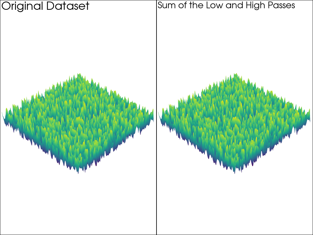
Low and High Pass identical to the original: True

Animate

Animate the variation of the cutoff frequency.

def warp_low_pass_noise(cfreq, scalar_ptp=sampled['scalars'].ptp()):
    """Process the sampled FFT and warp by scalars."""
    output = sampled_fft.low_pass(cfreq, cfreq, cfreq).rfft()

    # on the left: raw FFT magnitude
    output['scalars'] = output.active_scalars.real
    warped_raw = output.warp_by_scalar()

    # on the right: scale to fixed warped height
    output_scaled = output.translate((-11, 11, 0), inplace=False)
    output_scaled['scalars_warp'] = output['scalars'] / output['scalars'].ptp() * scalar_ptp
    warped_scaled = output_scaled.warp_by_scalar('scalars_warp')
    warped_scaled.active_scalars_name = 'scalars'
    # push center back to xy plane due to peaks near 0 frequency
    warped_scaled.translate((0, 0, -warped_scaled.center[-1]), inplace=True)

    return warped_raw + warped_scaled


# Initialize the plotter and plot off-screen to save the animation as a GIF.
plotter = pv.Plotter(notebook=False, off_screen=True)
plotter.open_gif("low_pass.gif", fps=8)

# add the initial mesh
init_mesh = warp_low_pass_noise(1e-2)
plotter.add_mesh(init_mesh, show_scalar_bar=False, lighting=False, n_colors=128)
plotter.camera.zoom(1.3)

for freq in np.geomspace(1e-2, 10, 25):
    plotter.clear()
    mesh = warp_low_pass_noise(freq)
    plotter.add_mesh(mesh, show_scalar_bar=False, lighting=False, n_colors=128)
    plotter.add_text(f"Cutoff Frequency: {freq:.2f}", color="black")
    plotter.write_frame()

# write the last frame a few times to "pause" the gif
for _ in range(10):
    plotter.write_frame()

plotter.close()

The left mesh in the above animation warps based on the raw values of the FFT amplitude. This emphasizes how taking into account more and more frequencies as the animation progresses, we recover a gradually larger proportion of the full noise sample. This is why the mesh starts “flat” and grows larger as the frequency cutoff is increased.

In contrast, the right mesh is always warped to the same visible height, irrespective of the cutoff frequency. This highlights how the typical wavelength (size of the features) of the Perlin noise decreases as the frequency cutoff is increased since wavelength and frequency are inversely proportional.