Visualize Hertzian Contact Stress

The following example demonstrates how to use PyVista to visualize Hertzian contact stress between a cylinder and a flat plate.

This example loads a dataset, constructs a line to represent the point of contact between the cylinder and the block, and samples the stress along that line. Finally, it plots the dataset and the stress distribution.

Background Hertzian contact stress refers to the stress that occurs between two curved surfaces that are in contact with each other. It is named after Heinrich Rudolf Hertz, a German physicist who first described the phenomenon in the late 1800s. Hertzian contact stress is an important concept in materials science, engineering, and other fields where the behavior of materials under stress is a critical consideration.

import matplotlib.pyplot as plt
import numpy as np

import pyvista as pv
from pyvista import examples

Load the dataset

Start by loading the dataset using pyvista.examples module. This module provides access to a range of datasets, including FEA (finite element analysis) datasets that are useful for stress analysis.

mesh = examples.download_fea_hertzian_contact_cylinder()
mesh

Header

Data Arrays

UnstructuredGrid Information N Cells 132258 N Points 34185 X Bounds -0.000e+00, 2.000e-01 Y Bounds 0.000e+00, 2.500e-02 Z Bounds 0.000e+00, 3.000e-01 N Arrays 16

Name Field Type N Comp Min Max Displacement Points float64 3 -5.000e-04 2.945e-05 vonMises Points float64 1 1.316e+02 1.707e+09 Stress Points float64 6 -3.055e+09 5.274e+08 Strain Points float64 6 -1.937e-02 1.894e-02 PrincipalStress 1 Points float64 1 -1.787e+09 2.586e+08 PrincipalStress 2 Points float64 1 -2.594e+09 3.531e+07 PrincipalStress 3 Points float64 1 -3.078e+09 1.995e+06 PrincipalStrain 1 Points float64 1 -6.976e-04 1.448e-02 PrincipalStrain 2 Points float64 1 -1.145e-02 8.690e-04 PrincipalStrain 3 Points float64 1 -2.787e-02 -8.375e-10 StrainEnergyDensity Points float64 1 1.172e-07 2.307e+07 PlasticStrain Points float64 6 0.000e+00 0.000e+00 EquivalentPlasticStrain Points float64 1 0.000e+00 0.000e+00 Rank Cells float64 1 0.000e+00 1.500e+01 Material Cells float64 1 0.000e+00 1.000e+00 PartID Cells int32 1 1.000e+00 2.000e+00

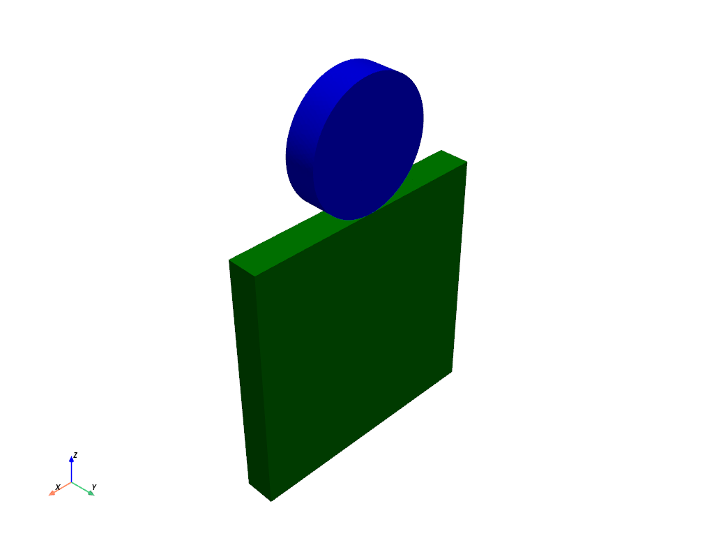
Plot the Dataset

Plot the dataset by part ID.

mesh.plot(scalars='PartID', cmap=['green', 'blue'], show_scalar_bar=False)

Static Scene

Interactive Scene

Creating a Line to Denote the Point of Contact

Construct a line to represent the point of contact between the cylinder and the plate.

ypos = 0.024
a = [0.1, ypos, 0.2 - 1e-4]
b = [0.095, ypos, 0.2 - 1e-4]
line = pv.Line(a, b, resolution=100)
line.clear_data()
line

PolyData	Information
N Cells	1
N Points	101
N Strips	0
X Bounds	9.500e-02, 1.000e-01
Y Bounds	2.400e-02, 2.400e-02
Z Bounds	1.999e-01, 1.999e-01
N Arrays	0

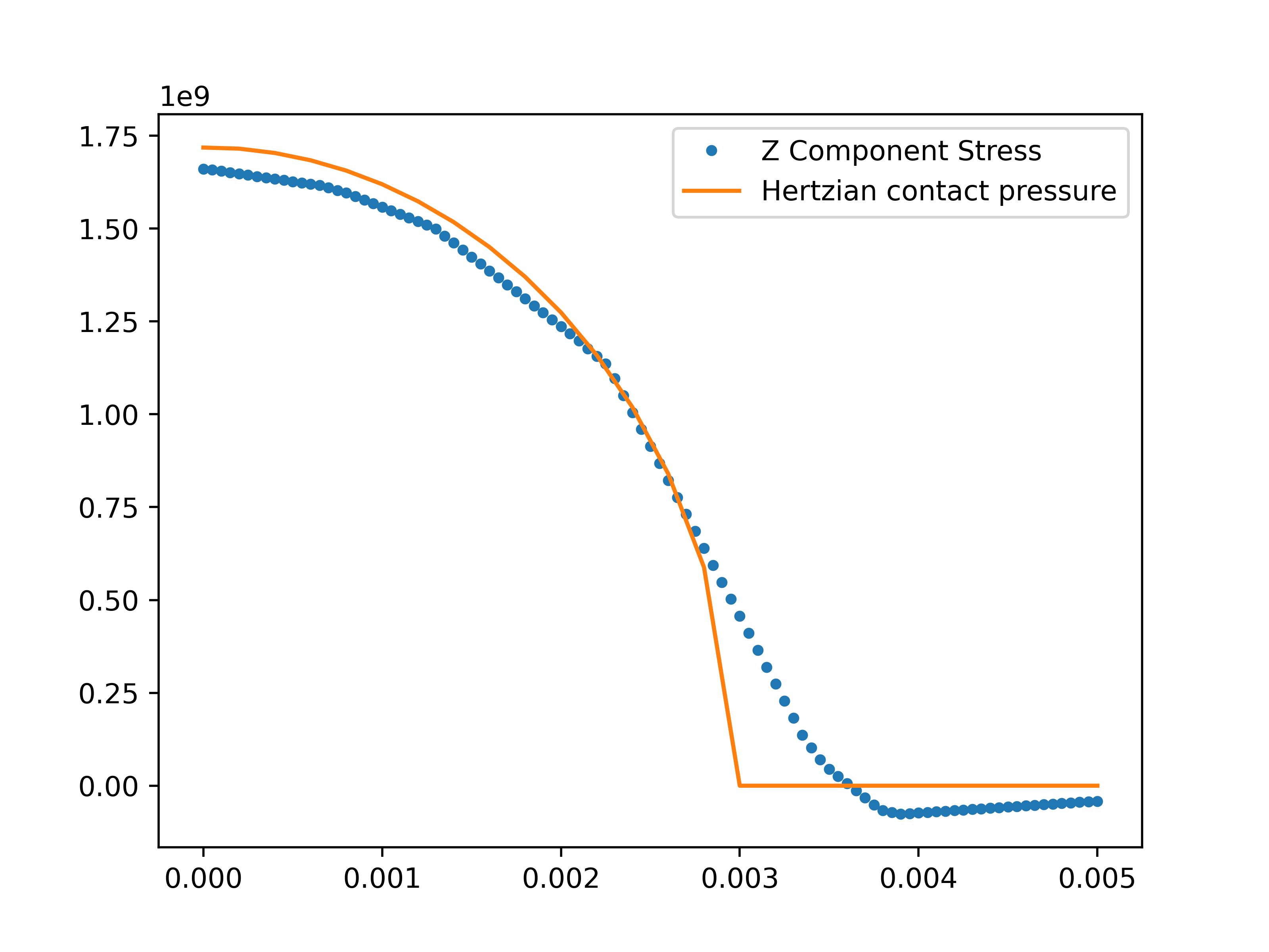
Sampling the Stress along the Line

We can sample the Z component stress along the contact edge and compare it with expected pressure.

The expected values array is the Hertzian contact pressure and is the analytical solution to the non-adhesive contact problem. Computation of these values is an exercise left up to the reader (the radius of the cylinder is 0.05). See Contact Mechanics

# Sample the stress
sampled = line.sample(mesh, tolerance=1e-3)
x_coord = 0.1 - sampled.points[:, 0]
samp_z_stress = -sampled['Stress'][:, 2]

# Expected Hertzian contact pressure
h_pressure = np.array(
    [
        [0.0000, 1718094092],
        [0.0002, 1715185734],
        [0.0004, 1703502649],
        [0.0006, 1683850714],
        [0.0008, 1655946243],
        [0.001, 1619362676],
        [0.0012, 1573494764],
        [0.0014, 1517500856],
        [0.0016, 1450208504],
        [0.0018, 1369953775],
        [0.002, 1274289906],
        [0.0022, 1159408887],
        [0.0024, 1018830677],
        [0.0026, 839747409.8],
        [0.0028, 587969605.2],
        [0.003, 0],
        [0.005, 0],
    ]
)

plt.plot(x_coord, samp_z_stress, '.', label='Z Component Stress')
plt.plot(h_pressure[:, 0], h_pressure[:, 1], label='Hertzian contact pressure')
plt.legend()
plt.show()

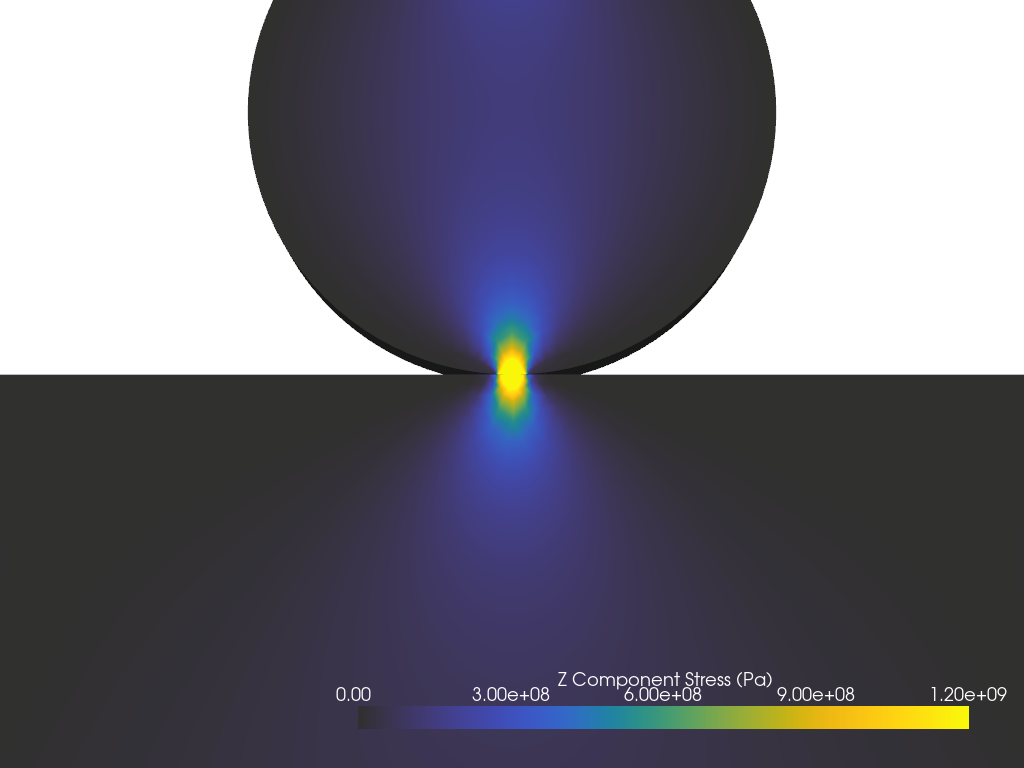
Visualizing the Z Stress Distribution

You can now visualize the Z stress distribution. Use pyvista.Plotter to create a plot window and add the dataset to it.

pl = pv.Plotter()
z_stress = np.abs(mesh['Stress'][:, 2])
pl.add_mesh(
    mesh,
    scalars=z_stress,
    clim=[0, 1.2e9],
    cmap='gouldian',
    scalar_bar_args={'title': 'Z Component Stress (Pa)', 'color': 'w'},
    lighting=True,
    show_edges=False,
    ambient=0.2,
)
pl.camera_position = 'xz'
pl.set_focus(a)
pl.camera.zoom(2.5)
pl.show()

Static Scene

Interactive Scene