Note
Go to the end to download the full example code.
Create Sphere Mesh Multiple Ways#
This example shows how to create meshes in different ways.
from __future__ import annotations

import numpy as np

import pyvista as pv
Simple Sphere#
The quickest method to get a Sphere mesh is to use pyvista.Sphere().
mesh = pv.Sphere()
mesh.plot(show_edges=True)
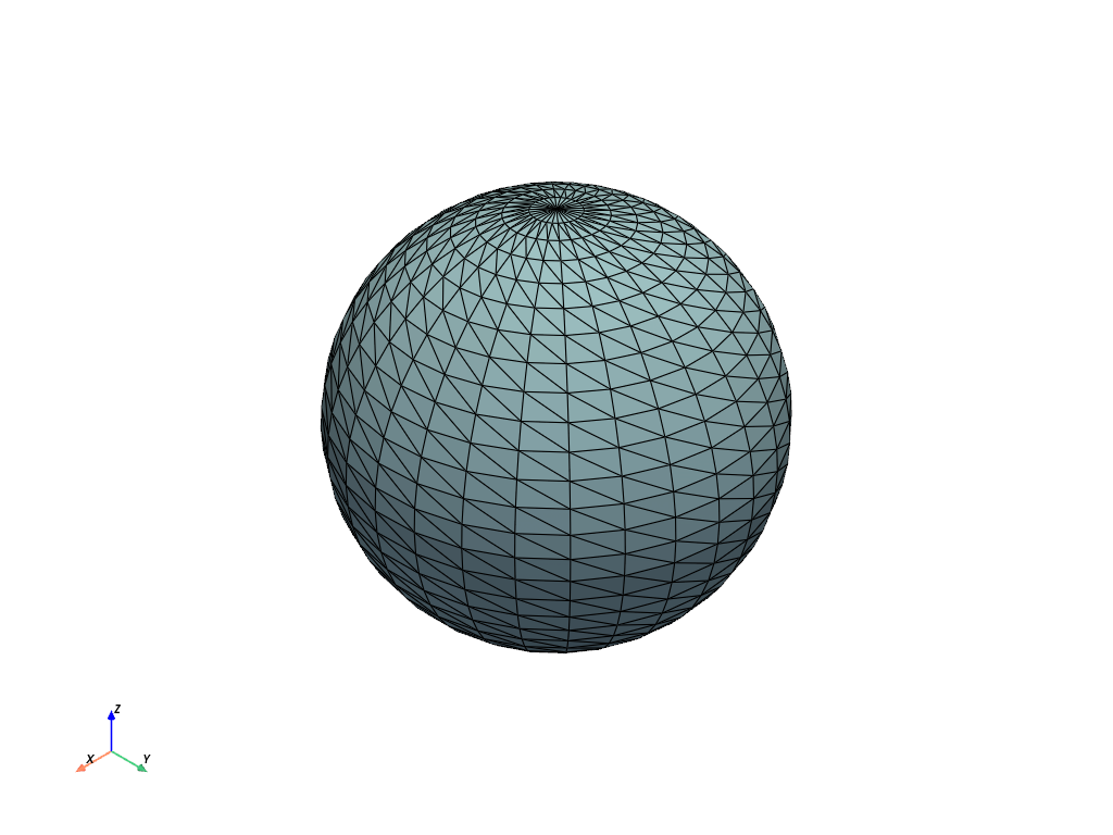
This gives an pyvista.PolyData mesh, i.e. a 2D surface.
mesh
In this case, it is manifold and
encloses a volume. To demonstrate this, there are no boundaries on the mesh
as indicated by no points/cells being extracted.
boundaries = mesh.extract_feature_edges(
    non_manifold_edges=True, feature_edges=False, manifold_edges=False
)
boundaries
The cells are TRIANGLE cells. For example, the first cell
mesh.get_cell(0).type
<CellType.TRIANGLE: 5>
Structured quadrilateral mesh of Sphere#
The structure of the mesh can be important. Instead of a triangulated mesh, it can be useful to have a structured mesh that has an i-j-k ordering that allows for simplified cell connectivity.
The points are generated as a regular grid in spherical coordinates using pyvista.spherical_to_cartesian().
Here, we will used the convention that theta is the
azimuthal angle, similar to longitude on the globe. phi is the
polar angle, similar to latitude on the globe.
The mesh has QUAD cells. The cells that look triangular
at the poles are actually degenerate quadrilaterals, i.e. two
points are coincident at the pole, as will be shown later.
mesh.plot(show_edges=True)

The mesh is of type pyvista.StructuredGrid.
mesh
The first cell is at the top pole, and it is a QUAD cell.
cell = mesh.get_cell(0)
cell.type
<CellType.QUAD: 9>
The first cell has two degenerate points.
cell.points
array([[0.        , 0.        , 0.5       ],
       [0.14086628, 0.        , 0.47974649],
       [0.0996075 , 0.0996075 , 0.47974649],
       [0.        , 0.        , 0.5       ]])
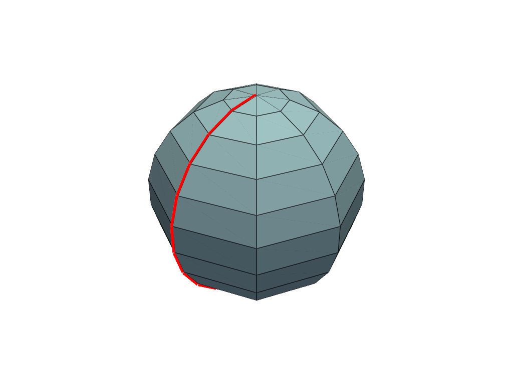
The cells on either side of the ‘seam’ along the start and end of the azimuthal component are not connected. These can be detected by extracting the boundary edges.
boundaries = mesh.extract_feature_edges(
    non_manifold_edges=True, feature_edges=False, manifold_edges=False
)
boundaries
Visualize this by plotting the boundary edges of the mesh.
pl = pv.Plotter()
pl.add_mesh(mesh, show_edges=True)
pl.add_mesh(boundaries, line_width=10, color='red')
pl.show()
Generate quadrilateral mesh of Sphere#
This example shows how a more complicated mesh can be defined.
In contrast to the example above, this example generates a mesh
that does not have degenerate points at the poles. TRIANGLE cells
will be used at the poles. First, regenerate the structured data.
We do not want duplicate points, so remove the duplicate in theta, which
results in 8 unique points in theta. Similarly, the poles at phi=0 and
phi=pi will be handled separately to avoid duplicate points, which
results in 10 unique points in phi. Remove these from the grid in spherical
coordinates.
Use pyvista.spherical_to_cartesian() to generate cartesian coordinates for points in the (N, 3)
format required by PyVista. Note that this method results in
the theta variable changing the fastest.
The first and last points are the poles.
First we will generate the cell-point connectivity similar to the
previous examples. At the poles, we will form triangles with the pole
and two adjacent points from the closest ring of points at a given phi
position. Otherwise, we will form quadrilaterals between two adjacent points
on consecutive phi positions.
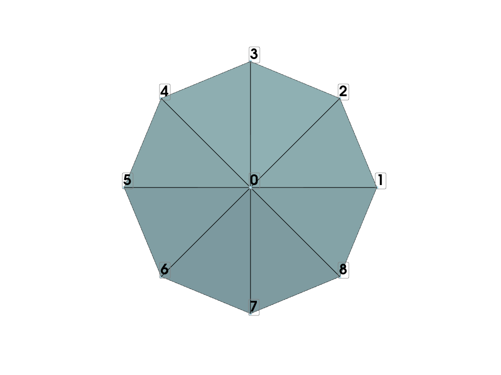
The first triangle in the mesh is point id 0, i.e. the pole, and
the first two points at the first phi position, id’s 1 and 2.
the next triangle contains the pole again and the next set of points,
id’s 2 and 3 and so on. The last point in the ring, id 8 connects
to the first point in the ring, 1, to form the last triangle. Exclude it
from the loop and add separately.
Demonstrate the connectivity of the mesh so far.
points_to_label = tuple(range(ntheta + 1))
mesh = pv.PolyData(points, faces=faces)
pl = pv.Plotter()
pl.add_mesh(mesh, show_edges=True)
pl.add_point_labels(
mesh.points[points_to_label, :], points_to_label, font_size=30, fill_shape=False
)
pl.view_xy()
pl.show()
Next form the quadrilaterals. This process is the same except
by connecting points across two levels of phi. For point 1
and point 2, these are connected to point 9 and point 10. Note
for quadrilaterals it must be defined in a consistent direction.
Again, the last point(s) in the theta direction connect back to the
first point(s).
Demonstrate the connectivity of the mesh with first quad layer.
points_to_label = tuple(range(ntheta * 2 + 1))
mesh = pv.PolyData(points, faces=faces)
pl = pv.Plotter()
pl.add_mesh(mesh, show_edges=True)
pl.add_point_labels(
mesh.points[points_to_label, :],
points_to_label,
font_size=30,
fill_shape=False,
always_visible=True,
)
pl.view_xy()
pl.show()
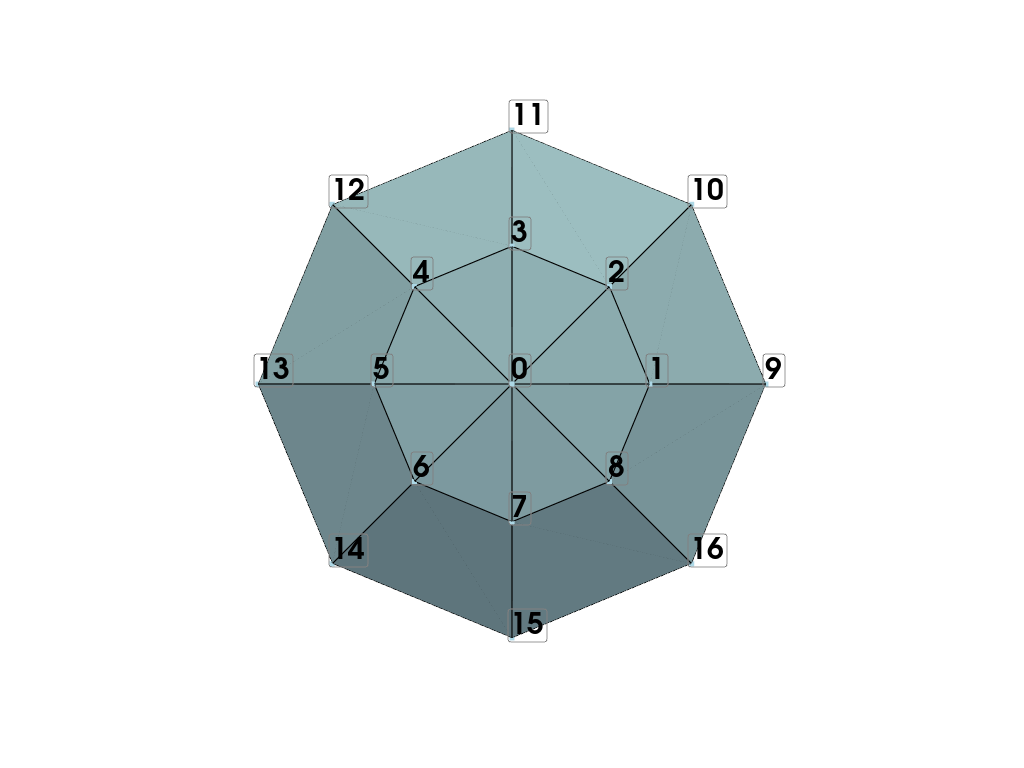
Next we loop over all adjacent levels of phi to form all the quadrilaterals and add the layer of triangles on the ending pole. Since we already formed the first layer of quadrilaterals, let’s start over to make cleaner code.
faces = []
for i in range(1, ntheta):
    faces.extend([3, 0, i, i + 1])

faces.extend([3, 0, ntheta, 1])
for j in range(nphi - 1):
for i in range(1, ntheta):
faces.extend(
[4, j * ntheta + i, j * ntheta + i + 1, i + (j + 1) * ntheta + 1, i + (j + 1) * ntheta]
)
faces.extend([4, (j + 1) * ntheta, j * ntheta + 1, (j + 1) * ntheta + 1, (j + 2) * ntheta])
for i in range(1, ntheta):
faces.extend([3, nphi * ntheta + 1, (nphi - 1) * ntheta + i, (nphi - 1) * ntheta + i + 1])
faces.extend([3, nphi * ntheta + 1, nphi * ntheta, (nphi - 1) * ntheta + 1])
We will use a pyvista.PolyData mesh here, but a
pyvista.UnstructuredGrid could also be used.
This mesh is manifold like pyvista.Sphere().
To demonstrate this, there are no boundaries on the mesh
as indicated by no points/cells being extracted.
boundaries = mesh.extract_feature_edges(
    non_manifold_edges=True, feature_edges=False, manifold_edges=False
)
boundaries
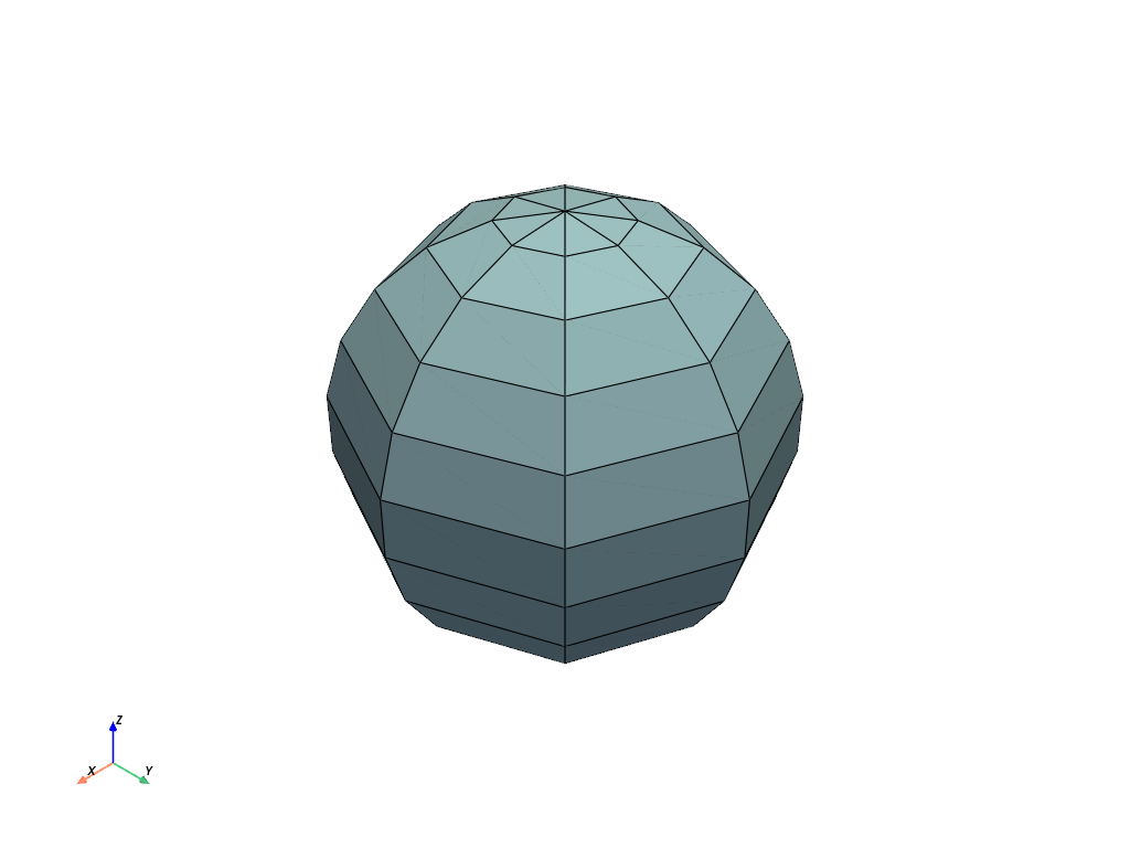
All the point labels are messy when plotted, so don’t add to the final plot.
mesh.plot(show_edges=True)
Total running time of the script: (0 minutes 1.182 seconds)
