Electronics Cooling CFD

Plot an electronics cooling CFD example from OpenFoam hosted on the public SimScale examples at SimScale Project Library and generated from the Thermal Management Tutorial: CHT Analysis of an Electronics Box.

This example dataset was read using the pyvista.POpenFOAMReader and post processed according to this README.md.

import numpy as np

import pyvista as pv
from pyvista import examples

Load the Datasets

Download and load the datasets.

The structure dataset consists of a box with several components, being cooled down by a fan, while the air dataset is the air, containing several scalar arrays including the velocity and temperature of the air.

structure, air = examples.download_electronics_cooling()
structure, air

(PolyData (0x7fd3e2dcd120)
  N Cells:    344270
  N Points:   187992
  N Strips:   0
  X Bounds:   -3.000e-03, 1.530e-01
  Y Bounds:   -3.000e-03, 2.030e-01
  Z Bounds:   -9.000e-03, 4.200e-02
  N Arrays:   4, UnstructuredGrid (0x7fd3646ef040)
  N Cells:    1749992
  N Points:   610176
  X Bounds:   -1.388e-18, 1.500e-01
  Y Bounds:   -3.000e-03, 2.030e-01
  Z Bounds:   -6.000e-03, 4.400e-02
  N Arrays:   10)

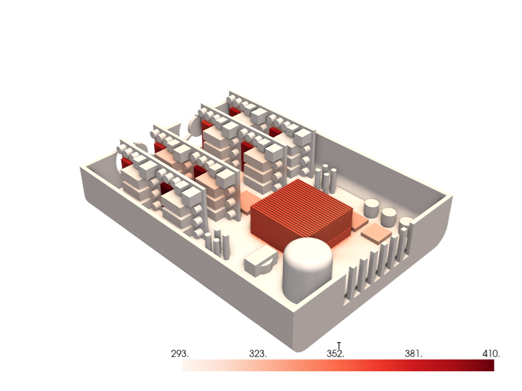
Plot the Electronics

Here we plot the temperature of the electronics using the "reds" colormap and improve the look of the plot using surface space ambient occlusion with enable_ssao().

pl = pv.Plotter()
pl.enable_ssao(radius=0.01)
pl.add_mesh(
    structure, scalars='T', smooth_shading=True, split_sharp_edges=True, cmap='reds', ambient=0.2
)
pl.enable_anti_aliasing('fxaa')  # also try 'ssaa'
pl.show()

Static Scene

Interactive Scene

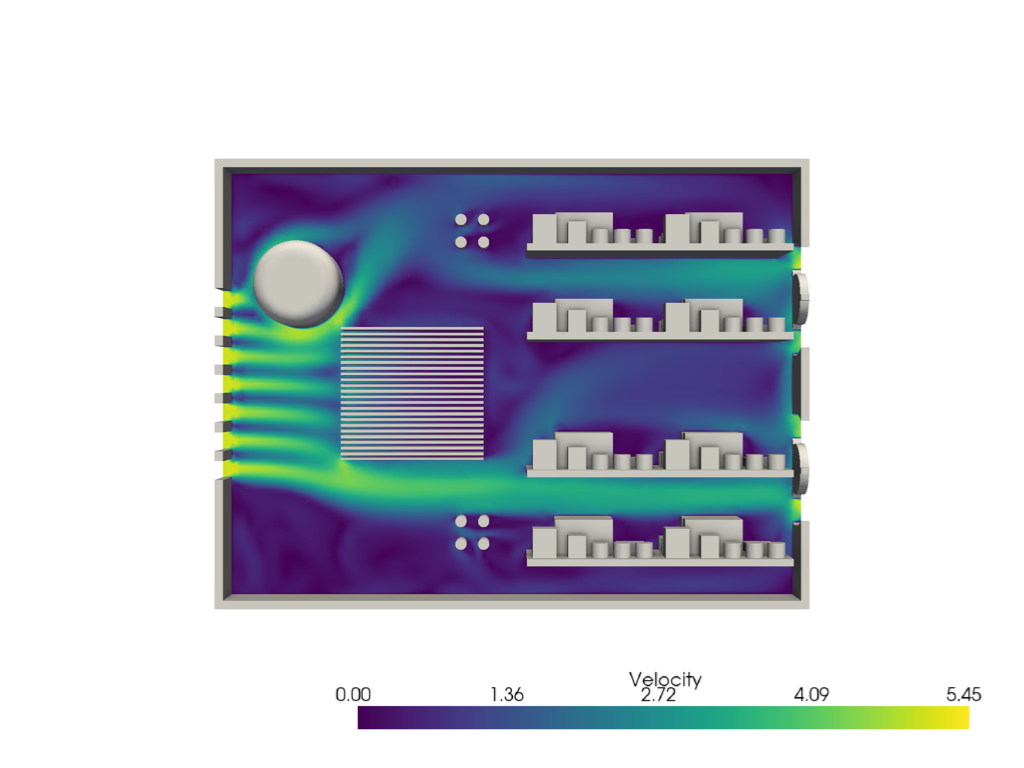
Plot Air Velocity

Let’s plot the velocity of the air.

Start by clipping the air dataset with clip() and plotting it alongside the electronics.

As you can see, the air enters from the front of the case (left) and is being pushed out of the “back” of the case via a fan.

# Clip the air in the XY plane
z_slice = air.clip('z', value=-0.005)

# Plot it
pl = pv.Plotter()
pl.enable_ssao(radius=0.01)
pl.add_mesh(z_slice, scalars='U', lighting=False, scalar_bar_args={'title': 'Velocity'})
pl.add_mesh(structure, color='w', smooth_shading=True, split_sharp_edges=True)
pl.camera_position = 'xy'
pl.camera.roll = 90
pl.enable_anti_aliasing('fxaa')
pl.show()

Static Scene

Interactive Scene

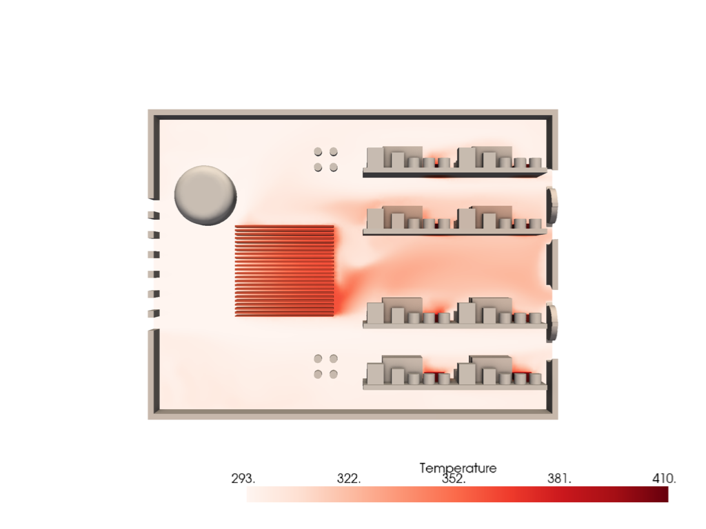
Plot Air Temperature

Let’s also plot the temperature of the air. This time, let’s also plot the temperature of the components.

pl = pv.Plotter()
pl.enable_ssao(radius=0.01)
pl.add_mesh(
    z_slice, scalars='T', lighting=False, scalar_bar_args={'title': 'Temperature'}, cmap='reds'
)
pl.add_mesh(
    structure,
    scalars='T',
    smooth_shading=True,
    split_sharp_edges=True,
    cmap='reds',
    show_scalar_bar=False,
)
pl.camera_position = 'xy'
pl.camera.roll = 90
pl.enable_anti_aliasing('fxaa')
pl.show()

Static Scene

Interactive Scene

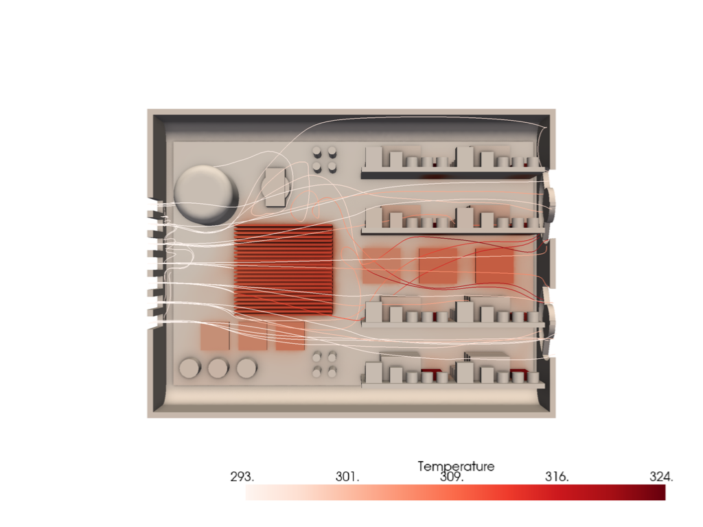
Plot Streamlines - Flow Velocity

Now, let’s plot the streamlines of this dataset so we can see how the air is flowing through the case.

Generate streamlines using streamlines_from_source().

# Have our streamlines start from the regular openings of the case.
points = []
for x in np.linspace(0.045, 0.105, 7, endpoint=True):
    points.extend([x, 0.2, z] for z in np.linspace(0, 0.03, 5))
points = pv.PointSet(points)
lines = air.streamlines_from_source(points, max_time=2.0)

# Plot
pl = pv.Plotter()
pl.enable_ssao(radius=0.01)
pl.add_mesh(lines, line_width=2, scalars='T', cmap='reds', scalar_bar_args={'title': 'Temperature'})
pl.add_mesh(
    structure,
    scalars='T',
    smooth_shading=True,
    split_sharp_edges=True,
    cmap='reds',
    show_scalar_bar=False,
)
pl.camera_position = 'xy'
pl.camera.roll = 90
pl.enable_anti_aliasing('fxaa')  # also try 'ssaa'
pl.show()

Static Scene

Interactive Scene

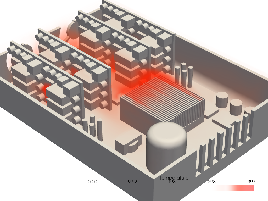
Volumetric Plot - Visualize High Temperatures

Show a 3D plot of areas of temperature.

For this example, we will first sample the results from the pyvista.UnstructuredGrid onto a pyvista.ImageData using sample(). This is so we can visualize it using add_volume()

bounds = np.array(air.bounds) * 1.2
origin = (bounds[0], bounds[2], bounds[4])
spacing = (0.002, 0.002, 0.002)
dimensions = (
    int((bounds[1] - bounds[0]) // spacing[0] + 2),
    int((bounds[3] - bounds[2]) // spacing[1] + 2),
    int((bounds[5] - bounds[4]) // spacing[2] + 2),
)
grid = pv.ImageData(dimensions=dimensions, spacing=spacing, origin=origin)
grid = grid.sample(air)

opac = np.zeros(20)
opac[1:] = np.geomspace(1e-7, 0.1, 19)
opac[-5:] = [0.05, 0.1, 0.5, 0.5, 0.5]

pl = pv.Plotter()
pl.add_mesh(structure, color='w', smooth_shading=True, split_sharp_edges=True)
vol = pl.add_volume(
    grid,
    scalars='T',
    opacity=opac,
    cmap='autumn_r',
    show_scalar_bar=True,
    scalar_bar_args={'title': 'Temperature'},
)
vol.prop.interpolation_type = 'linear'
pl.camera.zoom(2)
pl.show()