Plot Atomic Orbitals

Visualize the wave functions (orbitals) of the hydrogen atom.

Import

Import the applicable libraries.

Note

This example is modeled off of Matplotlib: Hydrogen Wave Function.

This example requires sympy. Install it with:

pip install sympy

import numpy as np

import pyvista as pv
from pyvista import examples

Generate the Dataset

Generate the dataset by evaluating the analytic hydrogen wave function from sympy.

\[\begin{equation} \psi_{n\ell m}(r,\theta,\phi) = \sqrt{ \left(\frac{2}{na_0}\right)^3\, \frac{(n-\ell-1)!}{2n[(n+\ell)!]} } e^{-r / na_0} \left(\frac{2r}{na_0}\right)^\ell L_{n-\ell-1}^{2\ell+1} \cdot Y_\ell^m(\theta, \phi) \end{equation}\]

See Hydrogen atom for more details.

This dataset evaluates this function for the hydrogen orbital \(3d_{xy}\), with the following quantum numbers:

• Principal quantum number: n=3

• Azimuthal quantum number: l=2

• Magnetic quantum number: m=-2

grid = examples.load_hydrogen_orbital(3, 2, -2)
grid

Header	Data Arrays
ImageData Information N Cells 970299 N Points 1000000 X Bounds -2.350e+01, 2.350e+01 Y Bounds -2.350e+01, 2.350e+01 Z Bounds -2.350e+01, 2.350e+01 Dimensions 100, 100, 100 Spacing 4.747e-01, 4.747e-01, 4.747e-01 N Arrays 2	Name Field Type N Comp Min Max real_wf Points float64 1 -1.689e-02 1.689e-02 wf Points complex128 1 -1.689e-02+1.353e-03j 1.689e-02+1.353e-03j

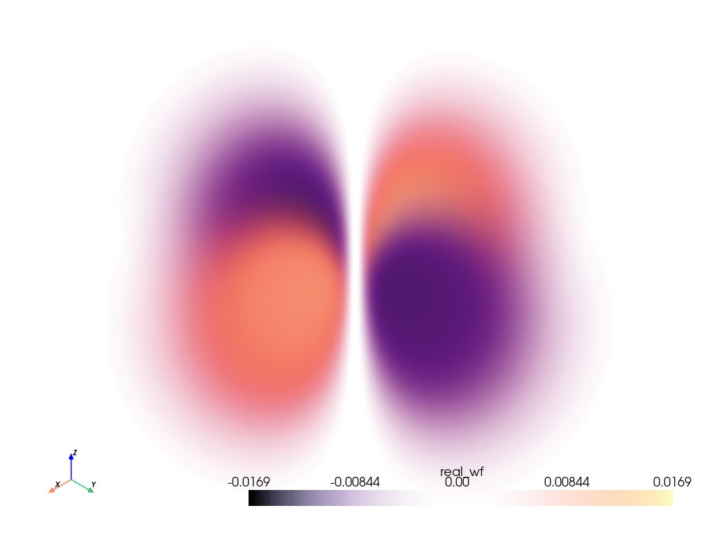
Plot the Orbital

Plot the orbital using add_volume() and using the default scalars contained in grid, real_wf. This way we can plot more than just the probability of the electron, but also the phase of the electron wave function.

Note

Since the real value of evaluated wave function for this orbital varies between [-<value>, <value>], we cannot use the default opacity opacity='linear'. Instead, we use [1, 0, 1] since we would like the opacity to be proportional to the absolute value of the scalars.

pl = pv.Plotter()
vol = pl.add_volume(grid, cmap='magma', opacity=[1, 0, 1])
vol.prop.interpolation_type = 'linear'
pl.camera.zoom(2)
pl.show_axes()
pl.show()

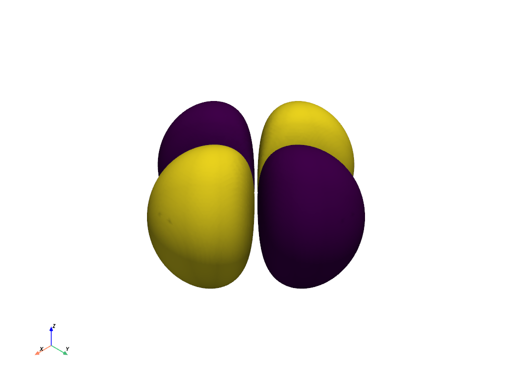
Plot the Orbital Contours as an Isosurface

Generate the contour plot for the orbital by determining when the orbital equals 10% the maximum value of the orbital. This effectively captures the most likely locations of the electron for this orbital.

Note how we use the absolute value of the scalars when evaluating contour() to capture where the positive and negative phases cross eval_at.

eval_at = grid['real_wf'].max() * 0.1
contours = grid.contour(
    [eval_at],
    scalars=np.abs(grid['real_wf']),
    method='marching_cubes',
)
contours = contours.interpolate(grid)
contours.plot(
    smooth_shading=True,
    show_scalar_bar=False,
)

Static Scene

Interactive Scene

Volumetric Plot: Plot the Orbitals using RGBA

Let’s now combine some of the best parts of the two above plots. The volumetric plot is great for showing the probability of the “electron cloud” orbitals, but the colormap doesn’t quite match reality as well as the isosurface plot.

For this example we’re going to use an RGBA colormap to tightly control the way the orbitals are plotted. For this, the opacity will be mapped to the probability of the electron being at a location in the grid, which we can do by taking the absolute value squared of the orbital’s wave function. We can set the color of the orbital based on the phase, which we can get simply with orbital['real_wf'] < 0.

Let’s start with a simple one, the \(3p_z\) orbital.

def plot_orbital(orbital, cpos='iso', clip_plane='x'):
    """Plot an electron orbital using an RGBA colormap."""
    neg_mask = orbital['real_wf'] < 0
    rgba = np.zeros((orbital.n_points, 4), np.uint8)
    rgba[neg_mask, 0] = 255
    rgba[~neg_mask, 1] = 255

    # normalize opacity
    opac = np.abs(orbital['real_wf']) ** 2
    opac /= opac.max()
    rgba[:, -1] = opac * 255

    orbital['plot_scalars'] = rgba

    pl = pv.Plotter()
    vol = pl.add_volume(
        orbital,
        scalars='plot_scalars',
    )
    vol.prop.interpolation_type = 'linear'
    if clip_plane:
        pl.add_volume_clip_plane(
            vol,
            normal=clip_plane,
            normal_rotation=False,
        )
    pl.camera_position = cpos
    pl.camera.zoom(1.5)
    pl.show_axes()
    return pl.show()


hydro_orbital = examples.load_hydrogen_orbital(3, 1, 0)
plot_orbital(hydro_orbital, clip_plane='-x')

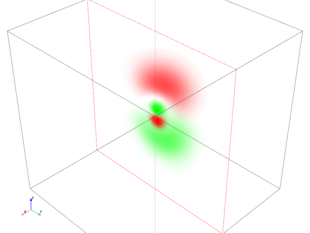
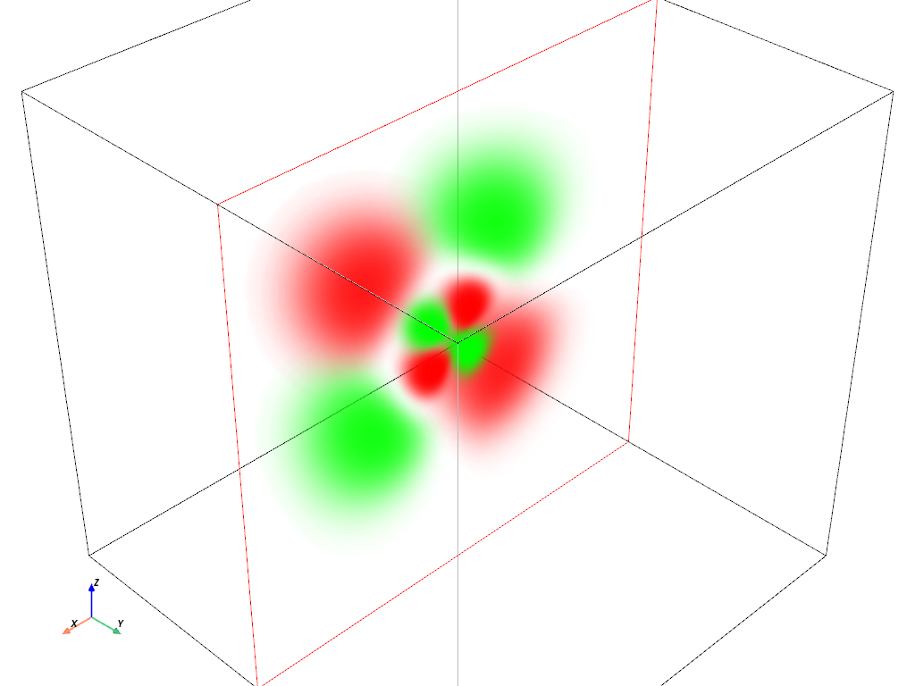
Volumetric Plot: \(4d_{z^2}\) orbital

hydro_orbital = examples.load_hydrogen_orbital(4, 2, 0)
plot_orbital(hydro_orbital, clip_plane='-y')

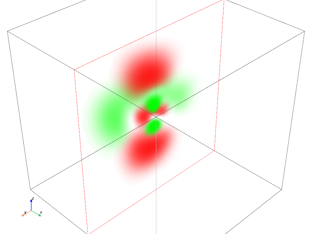
Volumetric Plot: \(4d_{xz}\) orbital

hydro_orbital = examples.load_hydrogen_orbital(4, 2, -1)
plot_orbital(hydro_orbital, clip_plane='-y')

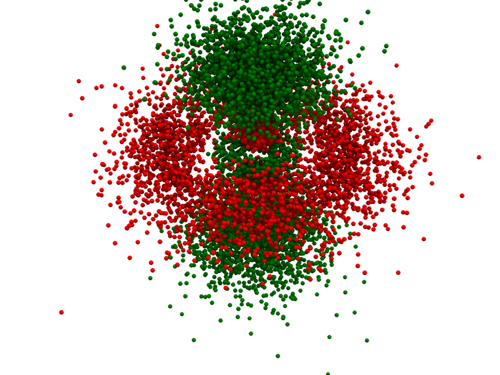
Plot an Orbital Using a Density Plot

We can also plot atomic orbitals using a 3D density plot. For this, we will use numpy.random.choice() to sample all the points of our pyvista.ImageData based on the probability of the electron being at that coordinate.

# Generate the orbital and sample based on the square of the probability of an
# electron being within a particular volume of space.
hydro_orbital = examples.load_hydrogen_orbital(4, 2, 0, zoom_fac=0.5)
prob = np.abs(hydro_orbital['real_wf']) ** 2
prob /= prob.sum()
indices = np.random.choice(hydro_orbital.n_points, 10000, p=prob)

# add a small amount of noise to these coordinates to remove the "grid like"
# structure present in the underlying ImageData
points = hydro_orbital.points[indices]
points += np.random.random(points.shape) - 0.5

# Create a point cloud and add the phase as the active scalars
point_cloud = pv.PolyData(points)
point_cloud['phase'] = hydro_orbital['real_wf'][indices] < 0

# Turn the point cloud into individual spheres. We do this so we can improve
# the plot by enabling surface space ambient occlusion (SSAO)
dplot = point_cloud.glyph(
    geom=pv.Sphere(theta_resolution=8, phi_resolution=8), scale=False, orient=False
)

# be sure to enable SSAO here. This makes the "points" that are deeper within
# the density plot darker.
pl = pv.Plotter()
pl.add_mesh(
    dplot,
    smooth_shading=True,
    show_scalar_bar=False,
    cmap=['red', 'green'],
    ambient=0.2,
)
pl.enable_ssao(radius=10)
pl.enable_anti_aliasing()
pl.camera.zoom(2)
pl.background_color = 'w'
pl.show()

Static Scene

Interactive Scene

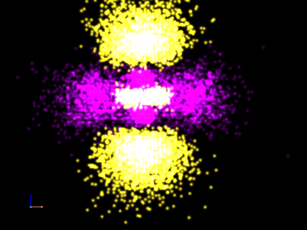
Density Plot - Gaussian Points Representation

Finally, let’s plot the same data using the “Gaussian points” representation.

point_cloud.plot(
    style='points_gaussian',
    render_points_as_spheres=False,
    point_size=3,
    emissive=True,
    background='k',
    show_scalar_bar=False,
    cpos='xz',
    zoom=2,
)