Compare Field Across Mesh Regions

Here is some velocity data from a glacier modelling simulation that is compared across nodes in the simulation. We have simplified the mesh to have the simulation node value already on the mesh.

This was originally posted to pyvista/pyvista-support#83.

The modeling results are courtesy of Urruty Benoit and are from the Elmer/Ice simulation software.

import numpy as np



import pyvista as pv
from pyvista import examples

# Load the sample data
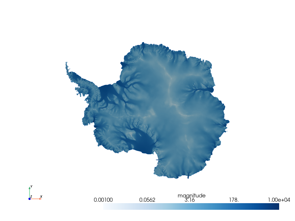
mesh = examples.download_antarctica_velocity()
mesh["magnitude"] = np.linalg.norm(mesh["ssavelocity"], axis=1)
mesh

Header	Data Arrays
PolyData Information N Cells 1106948 N Points 557470 N Strips 0 X Bounds -2.506e+06, 2.743e+06 Y Bounds -2.143e+06, 2.240e+06 Z Bounds 0.000e+00, 0.000e+00 N Arrays 3	Name Field Type N Comp Min Max ssavelocity Points float64 3 -4.341e+03 9.677e+03 node_value Points int64 1 0.000e+00 2.300e+01 magnitude Points float64 1 6.649e-03 1.013e+04

Here is a helper to extract regions of the mesh based on the simulation node.

def extract_node(node):
    idx = mesh["node_value"] == node
    return mesh.extract_points(idx)

p = pv.Plotter()
p.add_mesh(mesh, scalars="node_value")
for node in np.unique(mesh["node_value"]):
    loc = extract_node(node).center
    p.add_point_labels(loc, [f"Node {node}"])
p.show(cpos="xy")

vel_dargs = dict(scalars="magnitude", clim=[1e-3, 1e4], cmap='Blues', log_scale=True)

mesh.plot(cpos="xy", **vel_dargs)

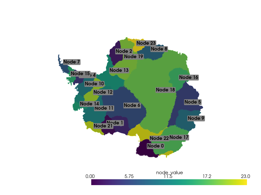
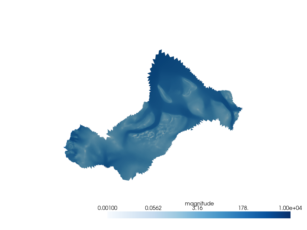
a = extract_node(12)
b = extract_node(20)

pl = pv.Plotter()
pl.add_mesh(a, **vel_dargs)
pl.add_mesh(b, **vel_dargs)
pl.show(cpos='xy')

plot vectors without mesh

pl = pv.Plotter()
pl.add_mesh(a.glyph(orient="ssavelocity", factor=20), **vel_dargs)
pl.add_mesh(b.glyph(orient="ssavelocity", factor=20), **vel_dargs)
pl.camera_position = [
    (-1114684.6969340036, 293863.65389149904, 752186.603224546),
    (-1114684.6969340036, 293863.65389149904, 0.0),
    (0.0, 1.0, 0.0),
]
pl.show()

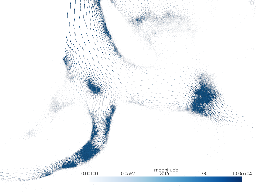
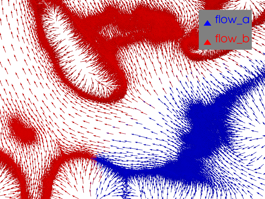
Compare directions. Normalize them so we can get a reasonable direction comparison.

flow_a = a.point_data['ssavelocity'].copy()
flow_a /= np.linalg.norm(flow_a, axis=1).reshape(-1, 1)
flow_b = b.point_data['ssavelocity'].copy()
flow_b /= np.linalg.norm(flow_b, axis=1).reshape(-1, 1)


# plot normalized vectors
pl = pv.Plotter()
pl.add_arrows(a.points, flow_a, mag=10000, color='b', label='flow_a')
pl.add_arrows(b.points, flow_b, mag=10000, color='r', label='flow_b')
pl.add_legend()
pl.camera_position = [
    (-1044239.3240694795, 354805.0268606294, 484178.24825854995),
    (-1044239.3240694795, 354805.0268606294, 0.0),
    (0.0, 1.0, 0.0),
]
pl.show()

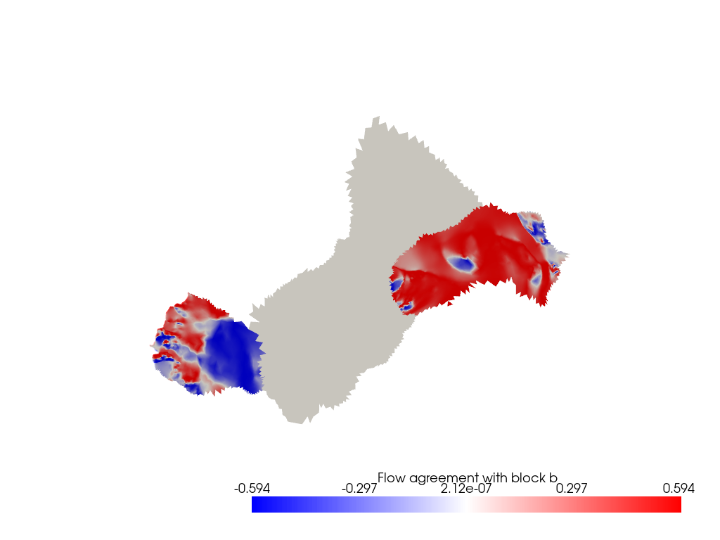
flow_a that agrees with the mean flow path of flow_b

agree = flow_a.dot(flow_b.mean(0))

pl = pv.Plotter()
pl.add_mesh(a, scalars=agree, cmap='bwr', scalar_bar_args={'title': 'Flow agreement with block b'})
pl.add_mesh(b, color='w')
pl.show(cpos='xy')

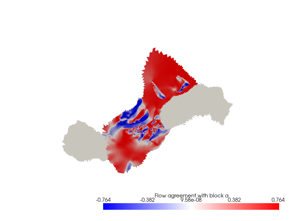
agree = flow_b.dot(flow_a.mean(0))

pl = pv.Plotter()
pl.add_mesh(a, color='w')
pl.add_mesh(b, scalars=agree, cmap='bwr', scalar_bar_args={'title': 'Flow agreement with block a'})
pl.show(cpos='xy')