Using Common Filters

Using common filters like thresholding and clipping.

from __future__ import annotations

import pyvista as pv
from pyvista import examples

PyVista wrapped data objects have a suite of common filters ready for immediate use directly on the object. These filters include the following (see Filters for a complete list):

• slice: creates a single slice through the input dataset on a user defined plane

• slice_orthogonal: creates a MultiBlock dataset of three orthogonal slices

• slice_along_axis: creates a MultiBlock dataset of many slices along a specified axis

• threshold: Thresholds a dataset by a single value or range of values

• threshold_percent: Threshold by percentages of the scalar range

• clip: Clips the dataset by a user defined plane

• outline_corners: Outlines the corners of the data extent

• extract_geometry: Extract surface geometry

To use these filters, call the method of your choice directly on your data object:

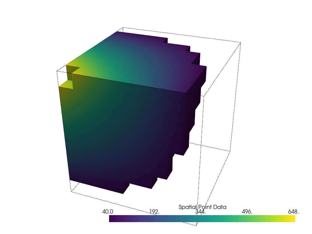
dataset = examples.load_uniform()
dataset.set_active_scalars('Spatial Point Data')

# Apply a threshold over a data range
threshed = dataset.threshold([100, 500])

outline = dataset.outline()

And now there is a thresholded version of the input dataset in the new threshed object. To learn more about what keyword arguments are available to alter how filters are executed, print the docstring for any filter attached to PyVista objects with either help(dataset.threshold) or using shift+tab in an IPython environment.

We can now plot this filtered dataset along side an outline of the original dataset

p = pv.Plotter()
p.add_mesh(outline, color='k')
p.add_mesh(threshed)
p.camera_position = [-2, 5, 3]
p.show()

Static Scene

Interactive Scene

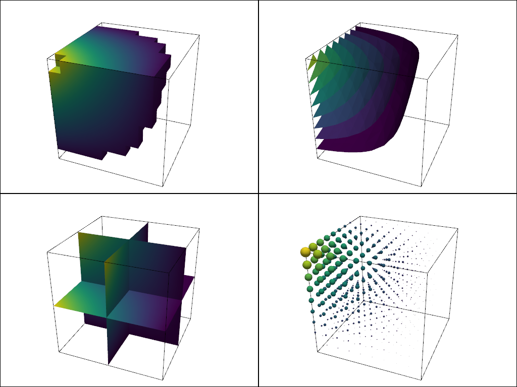
What about other filters? Let’s collect a few filter results and compare them:

contours = dataset.contour()
slices = dataset.slice_orthogonal()
glyphs = dataset.glyph(factor=1e-3, geom=pv.Sphere())

p = pv.Plotter(shape=(2, 2))
# Show the threshold
p.add_mesh(outline, color='k')
p.add_mesh(threshed, show_scalar_bar=False)
p.camera_position = [-2, 5, 3]
# Show the contour
p.subplot(0, 1)
p.add_mesh(outline, color='k')
p.add_mesh(contours, show_scalar_bar=False)
p.camera_position = [-2, 5, 3]
# Show the slices
p.subplot(1, 0)
p.add_mesh(outline, color='k')
p.add_mesh(slices, show_scalar_bar=False)
p.camera_position = [-2, 5, 3]
# Show the glyphs
p.subplot(1, 1)
p.add_mesh(outline, color='k')
p.add_mesh(glyphs, show_scalar_bar=False)
p.camera_position = [-2, 5, 3]

p.link_views()
p.show()

Static Scene

Interactive Scene

/home/runner/work/pyvista/pyvista/pyvista/core/filters/data_set.py:2695: UserWarning: No vector-like data to use for orient. orient will be set to False.
  warnings.warn('No vector-like data to use for orient. orient will be set to False.')

Filter Pipeline

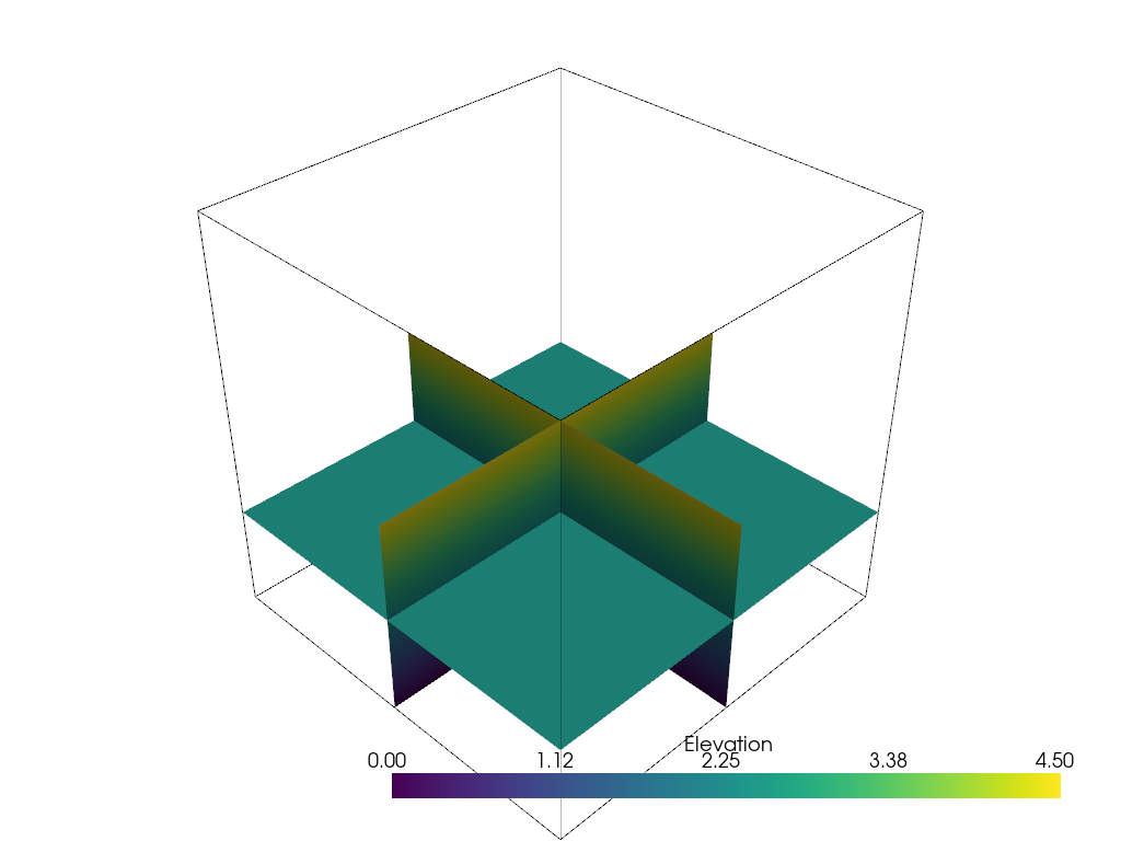
In VTK, filters are often used in a pipeline where each algorithm passes its output to the next filtering algorithm. In PyVista, we can mimic the filtering pipeline through a chain; attaching each filter to the last filter. In the following example, several filters are chained together:

1. First, and empty threshold filter to clean out any NaN values.

2. Use an elevation filter to generate scalar values corresponding to height.

3. Use the clip filter to cut the dataset in half.

4. Create three slices along each axial plane using the slice_orthogonal filter.

# Apply a filtering chain
result = dataset.threshold().elevation().clip(normal='z').slice_orthogonal()

And to view this filtered data, simply call the plot method (result.plot()) or create a rendering scene:

p = pv.Plotter()
p.add_mesh(outline, color='k')
p.add_mesh(result, scalars='Elevation')
p.view_isometric()
p.show()

Static Scene

Interactive Scene

Tags: filter