PyVista Data Model#
This section of the user guide explains in detail how to construct meshes from scratch and to utilize the underlying VTK data model but using the PyVista framework. Many of our Examples simply load data from files, but don’t explain how to construct meshes or place data within datasets.
Note
Though the following documentation section references VTK, it does not require that you have knowledge of VTK. For those who wish to see a detailed comparison to VTK or translate code written for the Python bindings of VTK to PyVista, please see Transitioning from VTK to PyVista.
For a more general description of our API, see What is a Mesh?.
The PyVista DataSet#
To visualize data in VTK or PyVista, two pieces of information are required: the data’s geometry, which describes where the data is positioned in space and what its values are, and its topology, which describes how points in the dataset are connected to one another.
At the top level, we have vtkDataObject, which are just “blobs” of data without geometry or topology. These contain arrays of vtkFieldData. Under this are vtkDataSet, which add geometry and topology to vtkDataObject. Associated with every point or cell in the dataset is a specific value. Since these values must be positioned and connected in space, they are held in the vtkDataArray class, which are simply memory buffers on the heap. In PyVista, 99% of the time we interact with vtkDataSet objects rather than with vtkDataObject objects. PyVista uses the same data types as VTK, but structures them in a more pythonic manner for ease of use.
If you’d like some background for how VTK structures its data, see Introduction to VTK in Python by Kitware, as well as the numerous code examples on Kitware’s GitHub site. An excellent introduction to mathematical concepts relevant to 3D modeling in general implemented in VTK is provided by the Discrete Differential Geometry YouTube Series by Prof. Keenan Crane at Carnegie Mellon. The concepts taught here will help improve your understanding of why data sets are structured the way they are in libraries like VTK.
At the most fundamental level, all PyVista geometry classes inherit from the Data Sets class. A dataset has geometry, topology, and attributes describing that geometry in the form of point, cell, or field arrays.
Geometry in PyVista is represented as points and cells. For example,
consider a single cell within a PolyData:
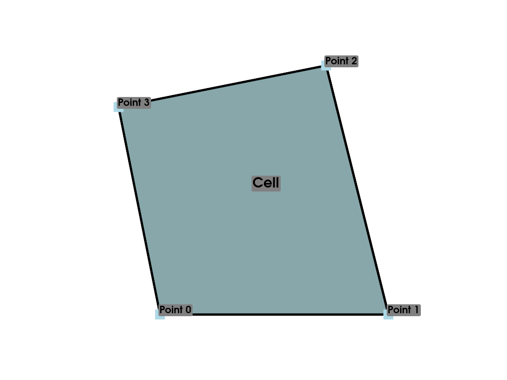
We would need a way to describe the position of each of these points in space, but we’re limited to expressing the values themselves as we’ve done above (lists of arrays with indices). VTK (and hence PyVista) have multiple classes that represent different data shapes. The most important dataset classes are shown below:
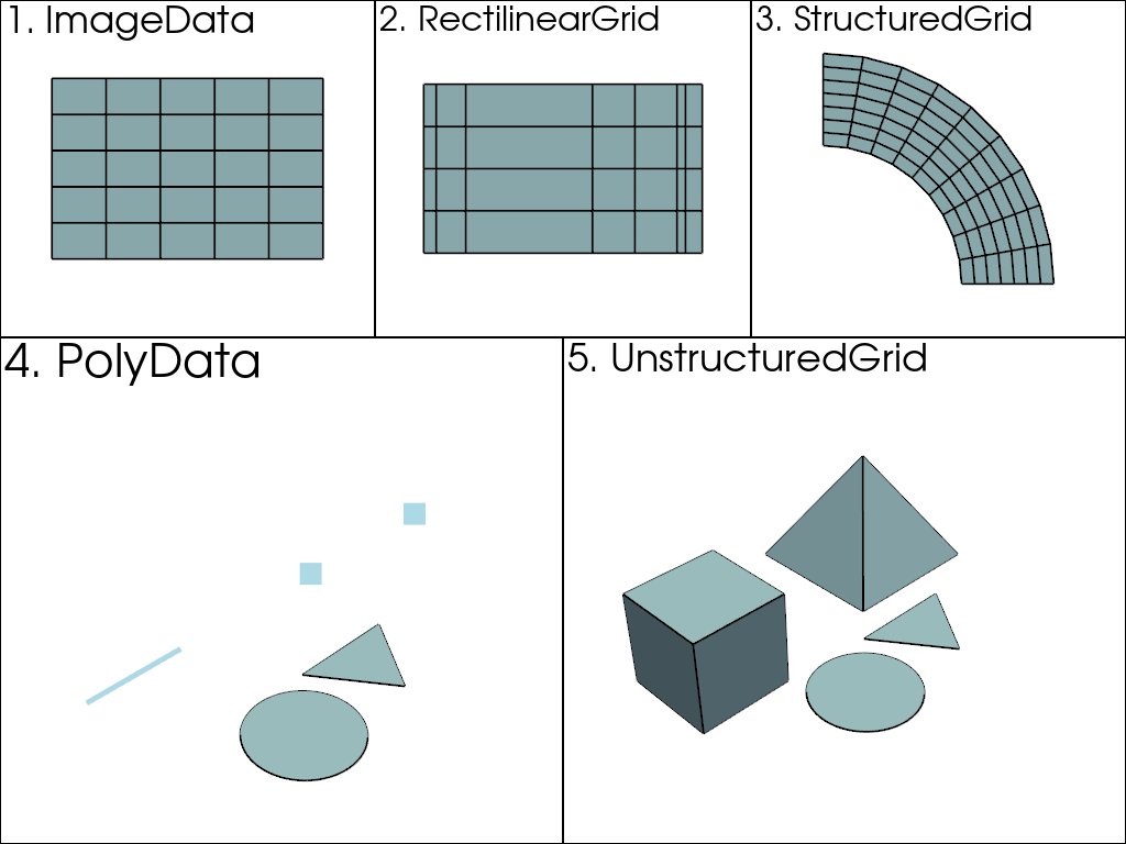
Here, the above datasets are ordered from most (5) to least complex
(1). That is, every dataset can be represented as an
UnstructuredGrid, but the
UnstructuredGrid class takes the most amount of
memory to store since they must account for every individual point and
cell . On the other hand, since vtkImageData
(ImageData) is uniformly spaced, a few integers and
floats can describe the shape, so it takes the least amount of memory
to store.
This is because in PolyData or
UnstructuredGrid, points, and cells must be explicitly
defined. In other data types, such as ImageData,
the cells (and even points) are defined as an emergent property based
on the dimensionality of the grid.
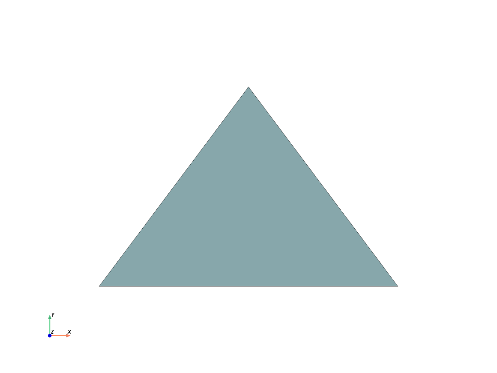
To see this in practice, let’s create the simplest surface represented
as a PolyData. First, we need to define our points.
Points and Arrays Within PyVista#
There are a variety of ways to create points within PyVista, and this section shows how to efficiently create an array of points by either:
Wrapping a VTK array
Using a
numpy.ndarrayOr just using a
list
PyVista provides pythonic methods for all three approaches so you can
choose whatever is most efficient for you. If you’re comfortable with
the VTK API, you can choose to wrap VTK arrays, but you may find that
using numpy.ndarray is more convenient and avoids the looping
overhead in Python.
Wrapping a VTK Array#
Let’s define points of a triangle. Using the VTK API, this can be done with:
>>> import vtk
>>> vtk_array = vtk.vtkDoubleArray()
>>> vtk_array.SetNumberOfComponents(3)
>>> vtk_array.SetNumberOfValues(9)
>>> vtk_array.SetValue(0, 0)
>>> vtk_array.SetValue(1, 0)
>>> vtk_array.SetValue(2, 0)
>>> vtk_array.SetValue(3, 1)
>>> vtk_array.SetValue(4, 0)
>>> vtk_array.SetValue(5, 0)
>>> vtk_array.SetValue(6, 0.5)
>>> vtk_array.SetValue(7, 0.667)
>>> vtk_array.SetValue(8, 0)
>>> print(vtk_array)
vtkDoubleArray (0x5624ddd9dd80)
  Debug: Off
  Modified Time: 83
  Reference Count: 1
  Registered Events: (none)
  Name: (none)
  Data type: double
  Size: 9
  MaxId: 8
  NumberOfComponents: 3
  Information: 0
  Name: (none)
  Number Of Components: 3
  Number Of Tuples: 3
  Size: 9
  MaxId: 8
  LookupTable: (none)
PyVista supports creating objects directly from the vtkDataArray
class, but there’s a better, and more pythonic alternative by using
numpy.ndarray.
Using NumPy with PyVista#
You can create a NumPy points array with:
>>> import numpy as np
>>> np_points = np.array([[0, 0, 0], [1, 0, 0], [0.5, 0.667, 0]])
>>> np_points
array([[0.   , 0.   , 0.   ],
       [1.   , 0.   , 0.   ],
       [0.5  , 0.667, 0.   ]])
We use a numpy.ndarray here so that PyVista directly “points”
the underlying C array to VTK. VTK already has APIs to directly read
in the C arrays from NumPy, and since VTK is written in C++,
everything from Python that is transferred over to VTK needs to be in a
format that VTK can process.
Should you wish to use VTK objects within PyVista, you can still do
this. In fact, using pyvista.wrap(), you can even get a numpy-like
representation of the data. For example:
>>> import pyvista as pv
>>> wrapped = pv.wrap(vtk_array)
>>> wrapped
pyvista_ndarray([[0.   , 0.   , 0.   ],
                 [1.   , 0.   , 0.   ],
                 [0.5  , 0.667, 0.   ]])
Note that when wrapping the underlying VTK array, we actually perform
a shallow copy of the data. In other words, we pass the pointer from
the underlying C array to the numpy.ndarray, meaning
that the two arrays are now efficiently linked (in NumPy terminology,
the returned array is a view into the underlying VTK data). This means
that we can change the array using numpy array indexing and have it
modified on the “VTK side”.
>>> wrapped[0, 0] = 10
>>> vtk_array.GetValue(0)
10.0
Or we can change the value from the VTK array and see it reflected in the numpy wrapped array. Let’s change the value back:
>>> vtk_array.SetValue(0, 0)
>>> wrapped[0, 0]
np.float64(0.0)
Using Python Lists or Tuples#
PyVista supports the use of Python sequences (that is, a list or
tuple), and you could define your points using a nested list
of lists via:
>>> points = [[0, 0, 0], [1, 0, 0], [0.5, 0.667, 0]]
When used in the context of PolyData to create the
mesh, this list will automatically be wrapped using NumPy and then
passed to VTK. This avoids any looping overhead and while still
allowing you to use native python classes.
Finally, let’s show how we can use these three objects in the context of a PyVista geometry class. Here, we create a simple point mesh containing just the three points:
>>> from_vtk = pv.PolyData(vtk_array)
>>> from_np = pv.PolyData(np_points)
>>> from_list = pv.PolyData(points)
These point meshes all contain three points and are effectively
identical. Let’s show this by accessing the underlying points array
from the mesh, which is represented as a pyvista.pyvista_ndarray
>>> from_vtk.points
pyvista_ndarray([[0.   , 0.   , 0.   ],
                 [1.   , 0.   , 0.   ],
                 [0.5  , 0.667, 0.   ]])
And show that these are all identical
>>> assert np.array_equal(from_vtk.points, from_np.points)
>>> assert np.array_equal(from_vtk.points, from_list.points)
>>> assert np.array_equal(from_np.points, from_list.points)
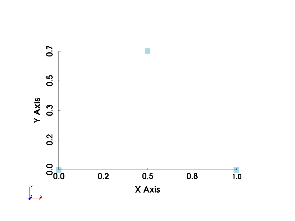
Finally, let’s plot this (very) simple example using PyVista’s
pyvista.plot() method. Let’s make this a full example so you
can see the entire process.
>>> import pyvista as pv
>>> points = [[0, 0, 0], [1, 0, 0], [0.5, 0.667, 0]]
>>> mesh = pv.PolyData(points)
>>> mesh.plot(show_bounds=True, cpos='xy', point_size=20)
We’ll get into PyVista’s data classes and attributes later, but for now we’ve shown how to create a simple geometry containing just points. To create a surface, we must specify the connectivity of the geometry, and to do that we need to specify the cells (or faces) of this surface.
Geometry and Mesh Connectivity/Topology Within PyVista#
With our previous example, we defined our “mesh” as three disconnected points. While this is useful for representing “point clouds,” if we want to create a surface, we have to describe the connectivity of the mesh. To do this, let’s define a single cell composed of three points in the same order as we defined earlier.
>>> cells = [3, 0, 1, 2]
Note
Observe how we had to insert a leading 3 to tell VTK that our
face is described by three elements, in this case, three points. In our PolyData VTK
doesn’t assume that faces always contain three points, so we have
to define that. This actually gives us the flexibility to define
as many (or as few as one) points per cell as we wish.
Note
All cell types follow the same connectivity array format:
[Number of points, Point 1, Point 2, ...]
Except for polyhedron type, in which we need to define each face of the cell. The
format for this type is the following:
[Number of elements, Number of faces, Face1NPoints, Point1, Point2, ..., PointN, Face2NPoints, ...].
Where number of elements is the total number of elements in the array that describe this cell.
Now we have all the necessary pieces to assemble an instance of
PolyData that contains a single triangle. To do
this, we simply provide the points and cells to the
constructor of a PolyData. We can see from the
representation that this geometry contains three points and one cell
>>> mesh = pv.PolyData(points, cells)
>>> mesh
PolyData (0x7f3c320b08e0)
  N Cells:    1
  N Points:   3
  N Strips:   0
  X Bounds:   0.000e+00, 1.000e+00
  Y Bounds:   0.000e+00, 6.670e-01
  Z Bounds:   0.000e+00, 0.000e+00
  N Arrays:   0
Let’s also plot this:
>>> mesh = pv.PolyData(points, [3, 0, 1, 2])
>>> mesh.plot(cpos='xy', show_edges=True)
While we’re at it, let’s annotate this plot to describe this mesh.
>>> pl = pv.Plotter()
>>> pl.add_mesh(mesh, show_edges=True, line_width=5)
>>> label_coords = mesh.points + [0, 0, 0.01]
>>> pl.add_point_labels(
...     label_coords,
...     [f'Point {i}' for i in range(3)],
...     font_size=20,
...     point_size=20,
...     always_visible=True,
... )
>>> pl.add_point_labels([0.43, 0.2, 0], ['Cell 0'], font_size=20)
>>> pl.camera_position = 'xy'
>>> pl.show()
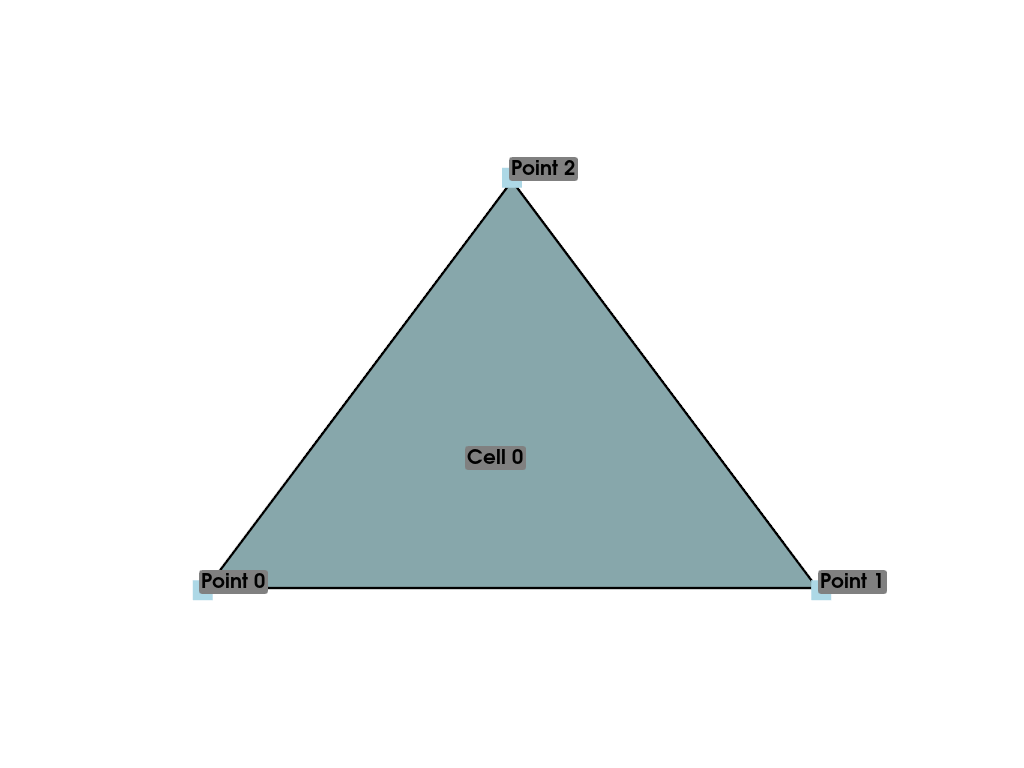
You can clearly see how the polygon is created based on the connectivity of the points.
This instance has several attributes to access the underlying data of
the mesh. For example, if you wish to access or modify the points of
the mesh, you can simply access the points attribute with
points.
>>> mesh.points
pyvista_ndarray([[0.   , 0.   , 0.   ],
                 [1.   , 0.   , 0.   ],
                 [0.5  , 0.667, 0.   ]])
The connectivity can also be accessed from the faces
attribute with:
>>> mesh.faces
array([3, 0, 1, 2])
Or we could simply get the representation of the mesh with:
>>> mesh
PolyData (0x7f3c320b08e0)
  N Cells:    1
  N Points:   3
  N Strips:   0
  X Bounds:   0.000e+00, 1.000e+00
  Y Bounds:   0.000e+00, 6.670e-01
  Z Bounds:   0.000e+00, 0.000e+00
  N Arrays:   0
In this representation we see:
Number of cells
n_cellsNumber of points
n_pointsBounds of the mesh
boundsNumber of data arrays
n_arrays
This is vastly different from the output from VTK. See Object Representation for the comparison between the two representations.
This mesh contains no data arrays as it consists only of geometry. This makes it useful for plotting just the geometry of the mesh, but datasets often contain more than just geometry. For example:
An electrical field computed from a changing magnetic field
Vector field of blood flow through artery
Surface stresses from a structural finite element analysis
Mineral deposits from geophysics
Weather patterns as a vector field or surface data.
While each one of these datasets could be represented as a different geometry class, they would all contain point, cell, or field data that explains the value of the data at a certain location within the geometry.
Data Arrays#
Each DataSet contains
attributes that allow you to access the underlying numeric data. This
numerical data may be associated with the points, cells, or not associated with points
or cells and attached to the mesh in general.
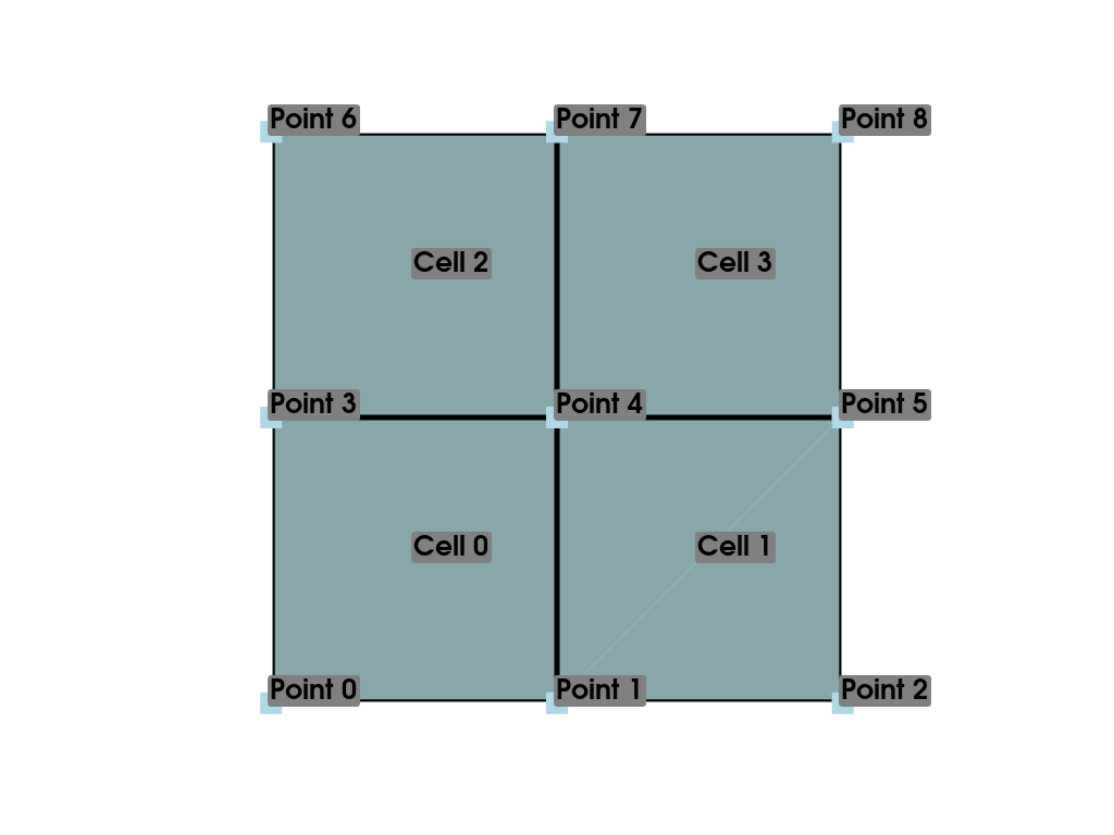
To illustrate data arrays within PyVista, let’s first construct a
slightly more complex mesh than our previous example. Here, we create
a simple mesh containing four isometric cells by starting with a
ImageData and then casting it to an UnstructuredGrid with
cast_to_unstructured_grid().
>>> grid = pv.ImageData(dimensions=(3, 3, 1))
>>> ugrid = grid.cast_to_unstructured_grid()
>>> ugrid
UnstructuredGrid (0x7f3c320b1a20)
  N Cells:    4
  N Points:   9
  X Bounds:   0.000e+00, 2.000e+00
  Y Bounds:   0.000e+00, 2.000e+00
  Z Bounds:   0.000e+00, 0.000e+00
  N Arrays:   0
Let’s also plot this basic mesh:
>>> pl = pv.Plotter()
>>> pl.add_mesh(ugrid, show_edges=True, line_width=5)
>>> label_coords = ugrid.points + [0, 0, 0.02]
>>> point_labels = [f'Point {i}' for i in range(ugrid.n_points)]
>>> pl.add_point_labels(
...     label_coords, point_labels, font_size=25, point_size=20
... )
>>> cell_labels = [f'Cell {i}' for i in range(ugrid.n_cells)]
>>> pl.add_point_labels(ugrid.cell_centers(), cell_labels, font_size=25)
>>> pl.camera_position = 'xy'
>>> pl.show()
Now that we have a simple mesh to work with, we can start assigning it data. There are two main types of data that can be associated with a mesh: scalar data and vector data. Scalar data is single or multi-component data that is non directional and may include values like temperature, or in the case of multi-component data, RGBA values. Vector data has magnitude and direction and is represented as arrays containing three components per data point.
When plotting, we can easily display scalar data, but this data must
be “associated” with either points or cells. For example, we may wish
to assign values to the cells of our example mesh, which we can do by
accessing the cell_data
attribute of our mesh.
Cell Data#
The easiest way to add scalar data to a DataSet is to use the [] operator.
Continuing with our example above, let’s assign each cell a single
integer. We can do this using a Python list and making it
the same length as the number of cells in the
UnstructuredGrid. Or as an even simpler example, using a
range of the appropriate length. Here we create the range, add
it to the cell_data, and then access
it using the [] operator.
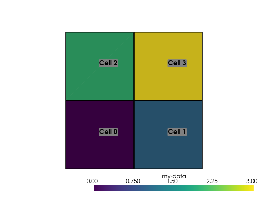
>>> simple_range = range(ugrid.n_cells)
>>> ugrid.cell_data['my-data'] = simple_range
>>> ugrid.cell_data['my-data']
pyvista_ndarray([0, 1, 2, 3])
Note how we are returned a pyvista.pyvista_ndarray. Since
VTK requires C arrays, PyVista will internally wrap or convert all
inputs to C arrays. We can then plot this with:
>>> ugrid.plot(cpos='xy', show_edges=True)
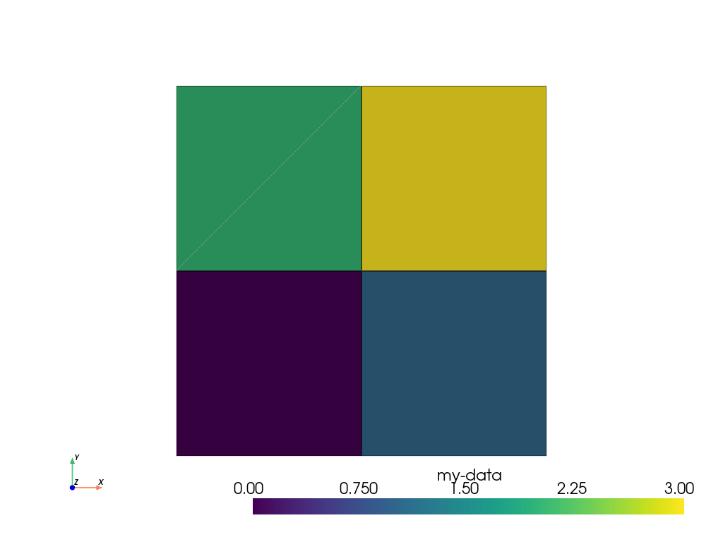
Note how we did not have to specify which cell data to plot as the
[] operator automatically sets the active scalars:
>>> ugrid.cell_data
pyvista DataSetAttributes
Association     : CELL
Active Scalars  : my-data
Active Vectors  : None
Active Texture  : None
Active Normals  : None
Contains arrays :
    my-data                 int64      (4,)                 SCALARS
We can also add labels to our plot to show which cells are assigned which scalars. Note how this is in the same order as the scalars we assigned.
>>> pl = pv.Plotter()
>>> pl.add_mesh(ugrid, show_edges=True, line_width=5)
>>> cell_labels = [f'Cell {i}' for i in range(ugrid.n_cells)]
>>> pl.add_point_labels(ugrid.cell_centers(), cell_labels, font_size=25)
>>> pl.camera_position = 'xy'
>>> pl.show()
We can continue to assign cell data to our DataSet using the [] operator, but if you
do not wish the new array to become the active array, you can add it
using set_array()
>>> data = np.linspace(0, 1, ugrid.n_cells)
>>> ugrid.cell_data.set_array(data, 'my-cell-data')
>>> ugrid.cell_data
pyvista DataSetAttributes
Association     : CELL
Active Scalars  : my-data
Active Vectors  : None
Active Texture  : None
Active Normals  : None
Contains arrays :
    my-data                 int64      (4,)                 SCALARS
    my-cell-data            float64    (4,)
Now, ugrid contains two arrays, one of which is the “active”
scalars. This set of active scalars will be the one plotted
automatically when scalars is unset in either add_mesh() or pyvista.plot(). This makes it
possible to have many cell arrays associated with a dataset and
track which one will plotted as the active cell scalars by default.
The active scalars can also be accessed via
active_scalars,
and the name of the active scalars array can be accessed or set with
active_scalars_name.
>>> ugrid.cell_data.active_scalars_name = 'my-cell-data'
>>> ugrid.cell_data
pyvista DataSetAttributes
Association     : CELL
Active Scalars  : my-cell-data
Active Vectors  : None
Active Texture  : None
Active Normals  : None
Contains arrays :
    my-data                 int64      (4,)
    my-cell-data            float64    (4,)                 SCALARS
Point Data#
Data can be associated to points in the same manner as in
Cell Data. The point_data attribute allows you to associate point
data to the points of a DataSet. Here, we will associate a simple
list to the points using the [] operator.
>>> simple_list = list(range(ugrid.n_points))
>>> ugrid.point_data['my-data'] = simple_list
>>> ugrid.point_data['my-data']
pyvista_ndarray([0, 1, 2, 3, 4, 5, 6, 7, 8])
Again, these values become the active scalars in our point arrays by
default by using the [] operator:
>>> ugrid.point_data
pyvista DataSetAttributes
Association     : POINT
Active Scalars  : my-data
Active Vectors  : None
Active Texture  : None
Active Normals  : None
Contains arrays :
    my-data                 int64      (9,)                 SCALARS
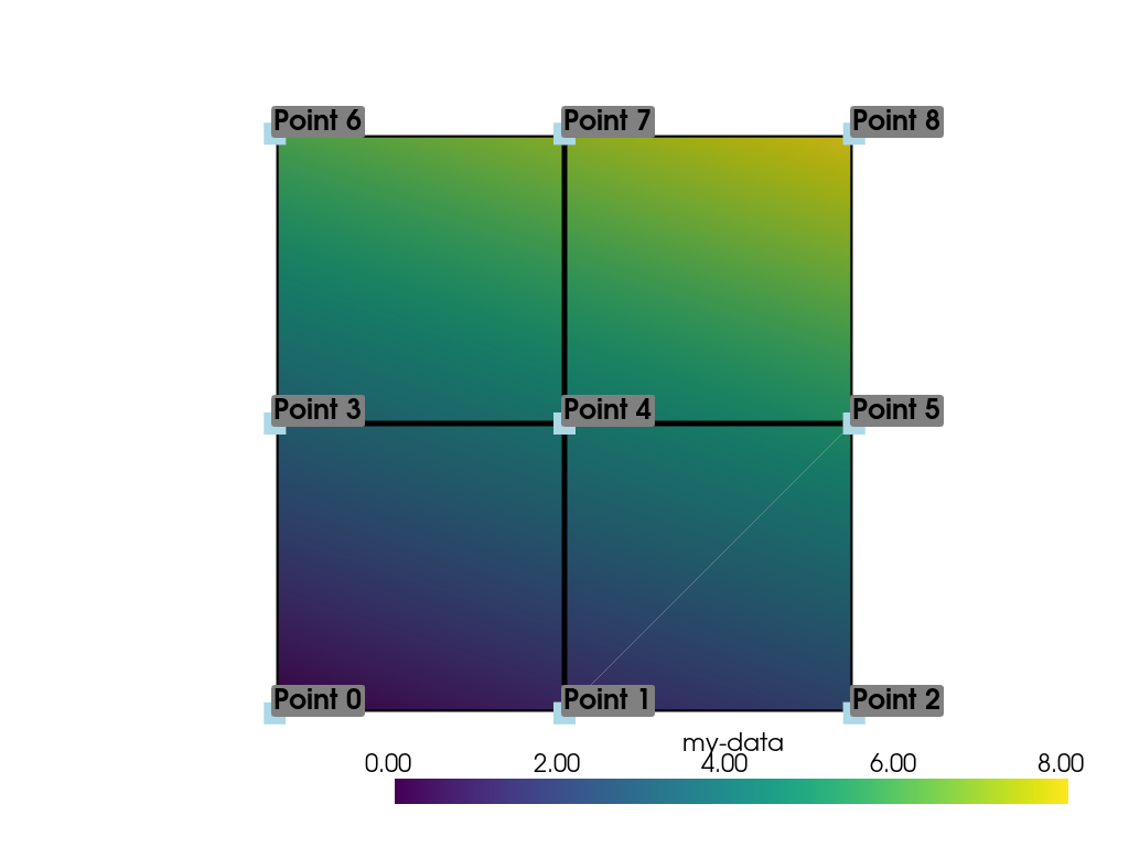
Let’s plot the point data. Note how this varies from the cell data
plot; each individual point is assigned a scalar value which is
interpolated across a cell to create a smooth color map between the
lowest value at Point 0 to the highest value at Point 8.
>>> pl = pv.Plotter()
>>> pl.add_mesh(ugrid, show_edges=True, line_width=5)
>>> label_coords = ugrid.points + [0, 0, 0.02]
>>> point_labels = [f'Point {i}' for i in range(ugrid.n_points)]
>>> pl.add_point_labels(
...     label_coords, point_labels, font_size=25, point_size=20
... )
>>> pl.camera_position = 'xy'
>>> pl.show()
As in Cell Data, we can assign multiple
arrays to point_data
using set_array().
>>> data = np.linspace(0, 1, ugrid.n_points)
>>> ugrid.point_data.set_array(data, 'my-point-data')
>>> ugrid.point_data
pyvista DataSetAttributes
Association     : POINT
Active Scalars  : my-data
Active Vectors  : None
Active Texture  : None
Active Normals  : None
Contains arrays :
    my-data                 int64      (9,)                 SCALARS
    my-point-data           float64    (9,)
Again, here there are now two arrays associated to the point data, and
only one is the “active” scalars array. Like as in the cell data, we
can retrieve this with active_scalars, and the name of the
active scalars array can be accessed or set with
active_scalars_name.
>>> ugrid.point_data.active_scalars_name = 'my-point-data'
>>> ugrid.point_data
pyvista DataSetAttributes
Association     : POINT
Active Scalars  : my-point-data
Active Vectors  : None
Active Texture  : None
Active Normals  : None
Contains arrays :
    my-data                 int64      (9,)
    my-point-data           float64    (9,)                 SCALARS
Dataset Active Scalars#
Continuing from the previous sections, our ugrid dataset now
contains both point and cell data:
>>> ugrid.point_data
pyvista DataSetAttributes
Association     : POINT
Active Scalars  : my-point-data
Active Vectors  : None
Active Texture  : None
Active Normals  : None
Contains arrays :
    my-data                 int64      (9,)
    my-point-data           float64    (9,)                 SCALARS
>>> ugrid.cell_data
pyvista DataSetAttributes
Association     : CELL
Active Scalars  : my-cell-data
Active Vectors  : None
Active Texture  : None
Active Normals  : None
Contains arrays :
    my-data                 int64      (4,)
    my-cell-data            float64    (4,)                 SCALARS
There are active scalars in both point and cell data, but only one
type of scalars can be “active” at the dataset level. The reason for
this is that only one scalar type (be it point or cell) can be plotted
at once, and this data can be obtained from active_scalars_info:
>>> ugrid.active_scalars_info
ActiveArrayInfoTuple(association=<FieldAssociation.POINT: 0>, name='my-point-data')
Note that the active scalars are by default the point scalars. You
can change this by setting the active scalars with
set_active_scalars(). Note that if you
want to set the active scalars and both the point and cell data have
an array of the same name, you must specify the preference:
>>> ugrid.set_active_scalars('my-data', preference='cell')
>>> ugrid.active_scalars_info
ActiveArrayInfoTuple(association=<FieldAssociation.CELL: 1>, name='my-data')
This can also be set when plotting using the preference
parameter in add_mesh() or
pyvista.plot().
Field Data#
Field arrays are different from point_data and cell_data in that they are not associated with
the geometry of the DataSet.
This means that while it’s not possible to designate the field data as
active scalars or vectors, you can use it to “attach” arrays of any
shape. You can even add string arrays in the field data:
>>> ugrid.field_data['my-field-data'] = ['hello', 'world']
>>> ugrid.field_data['my-field-data']
pyvista_ndarray(['hello', 'world'], dtype='<U5')
Note that the field data is automatically transferred to VTK C-style arrays and then represented as a numpy data format.
When listing the current field data, note that the association is “NONE”:
>>> ugrid.field_data
pyvista DataSetAttributes
Association     : NONE
Contains arrays :
    my-field-data           <U5        (2,)
This is because the data is not associated with points or cells, and cannot be made so because field data is not expected to match the number of cells or points. As such, it also cannot be plotted.
Vectors, Texture Coords, and Normals Attributes#
Both cell and point data can also store the following “special” attributes in addition to active_scalars:
Active Normals#
The active_normals array is a special array that
specifies the local normal direction of meshes. It is used for
creating physically based rendering, rendering smooth shading using
Phong interpolation, warping by scalars, etc. If this array
is not set when plotting with smooth_shading=True or pbr=True,
it will be computed.
Active Texture Coordinates#
The active_texture_coordinates array is used for
rendering textures. See Applying Textures for examples using
this array.
Active Vectors#
The active_vectors is an array containing
quantities that have magnitude and direction (specifically, three
components). For example, a vector field containing the wind speed at
various coordinates. This differs from active_scalars as scalars are expected
to be non-directional even if they contain several components (as in
the case of RGB data).
Vectors are treated differently within VTK than scalars when performing
transformations using the transform()
filter. Unlike scalar arrays, vector arrays will be transformed along
with the geometry as these vectors represent quantities with direction.
Note
VTK permits only one “active” vector. If you have multiple vector
arrays that you wish to transform, set transform_all_input_vectors=True
in transform(). Be aware that this
will transform any array with three components, so multi-component
scalar arrays like RGB arrays will have to be discarded after
transformation.