Note
Go to the end to download the full example code.
Applying Textures#
Plot a mesh with an image projected onto it as a texture.
from matplotlib.pyplot import get_cmap
import numpy as np
import pyvista as pv
from pyvista import examples
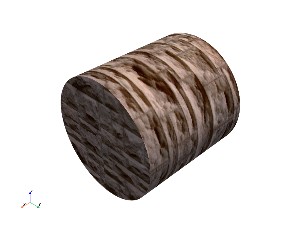
Texture mapping is easily implemented using PyVista. Many of the geometric objects come preloaded with texture coordinates, so quickly creating a surface and displaying an image is simply:
# load a sample texture
tex = examples.download_masonry_texture()

# create a surface to host this texture
surf = pv.Cylinder()

surf.plot(texture=tex)
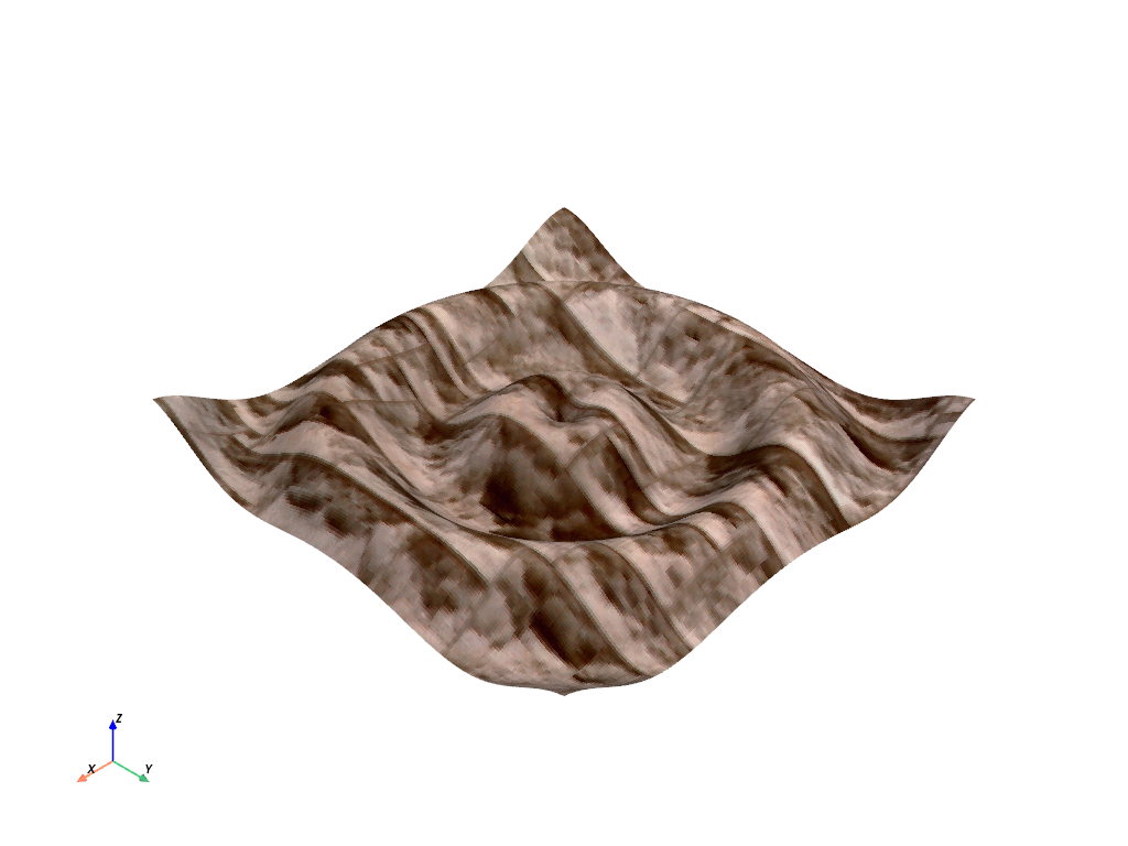
But what if your dataset doesn’t have texture coordinates? Then you can
harness the pyvista.DataSetFilters.texture_map_to_plane() filter to
properly map an image to a dataset’s surface.
For example, let’s map that same image of bricks to a curvey surface:
# create a structured surface
x = np.arange(-10, 10, 0.25)
y = np.arange(-10, 10, 0.25)
x, y = np.meshgrid(x, y)
r = np.sqrt(x**2 + y**2)
z = np.sin(r)
curvsurf = pv.StructuredGrid(x, y, z)

# Map the curved surface to a plane - use best fitting plane
curvsurf.texture_map_to_plane(inplace=True)

curvsurf.plot(texture=tex)
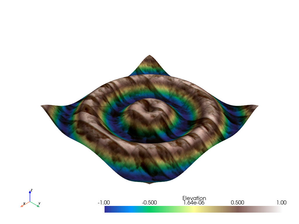
Display scalar data along with a texture by ensuring the
interpolate_before_map setting is False and specifying both the
texture and scalars arguments.
elevated = curvsurf.elevation()

elevated.plot(
    scalars='Elevation', cmap='terrain', texture=tex, interpolate_before_map=False
)
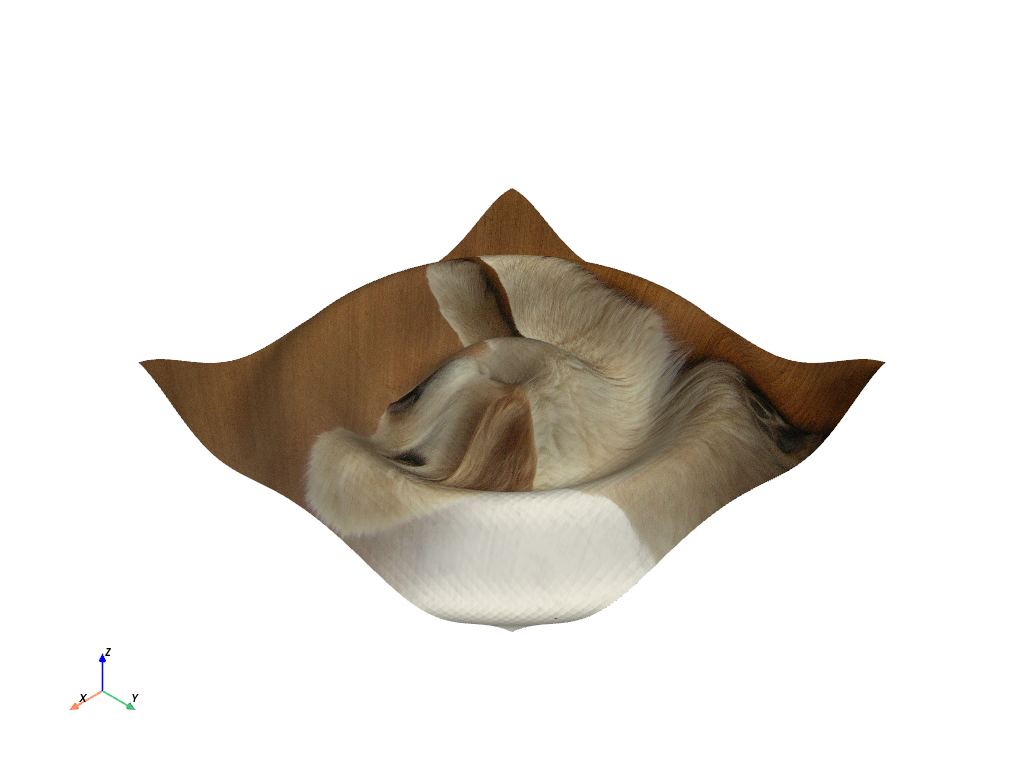
Note that this process can be completed with any image texture.
# use the puppy image
tex = examples.download_puppy_texture()
curvsurf.plot(texture=tex)
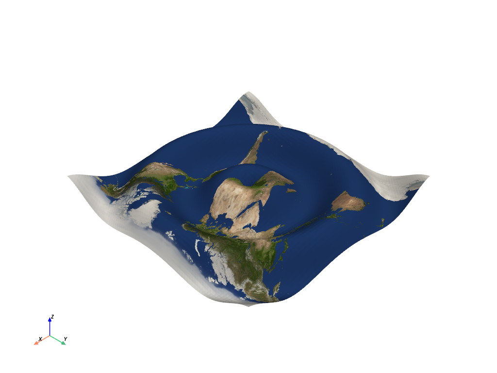
Textures from Files#
What about loading your own texture from an image? This is often most easily
done using the pyvista.read_texture() function - simply pass an image
file’s path, and this function with handle making a vtkTexture for you to
use.
image_file = examples.mapfile
tex = pv.read_texture(image_file)
curvsurf.plot(texture=tex)
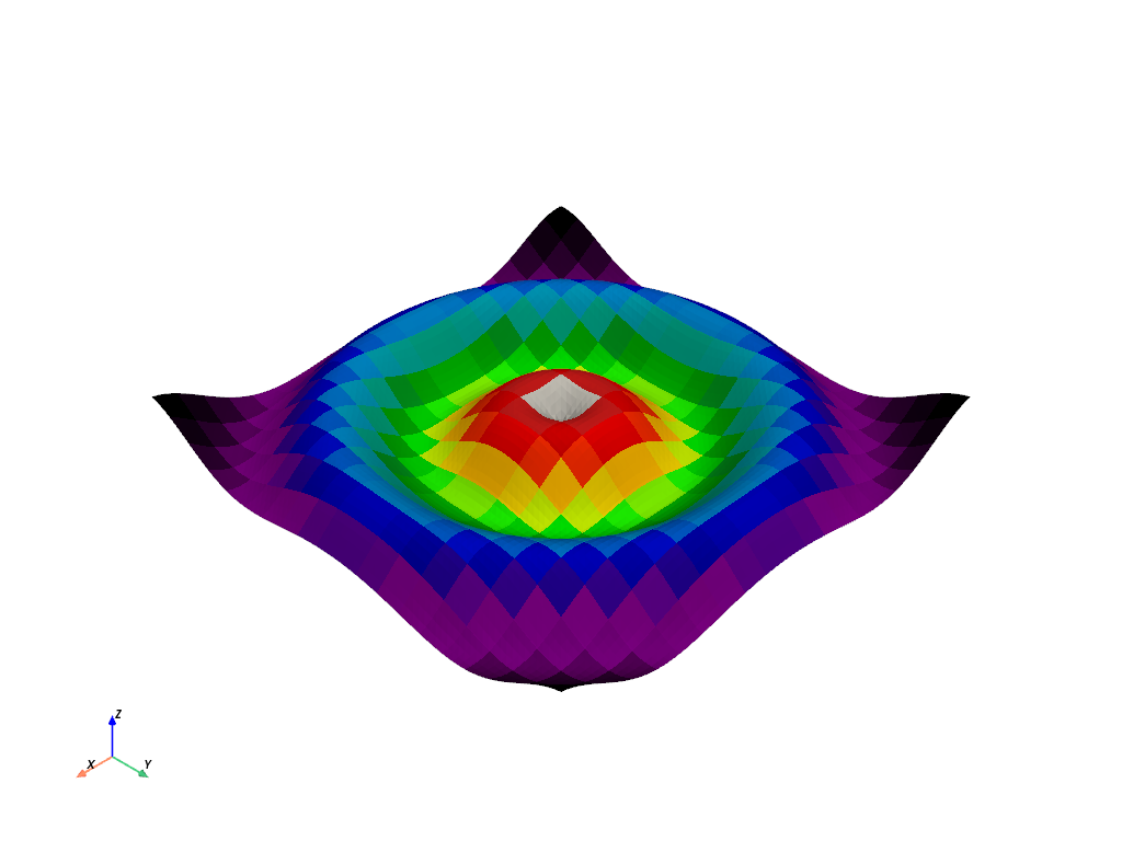
NumPy Arrays as Textures#
Want to use a programmatically built image? pyvista.ImageData
objects can be converted to textures using pyvista.image_to_texture()
and 3D NumPy (X by Y by RGB) arrays can be converted to textures using
pyvista.numpy_to_texture().
# create an image using numpy,
xx, yy = np.meshgrid(np.linspace(-200, 200, 20), np.linspace(-200, 200, 20))
A, b = 500, 100
zz = A * np.exp(-0.5 * ((xx / b) ** 2.0 + (yy / b) ** 2.0))

# Creating a custom RGB image
cmap = get_cmap('nipy_spectral')
norm = lambda x: (x - np.nanmin(x)) / (np.nanmax(x) - np.nanmin(x))
hue = norm(zz.ravel())
colors = (cmap(hue)[:, 0:3] * 255.0).astype(np.uint8)
image = colors.reshape((xx.shape[0], xx.shape[1], 3), order='F')

# Convert 3D numpy array to texture
tex = pv.numpy_to_texture(image)

# Render it
curvsurf.plot(texture=tex)
Create a GIF Movie with updating textures#
Generate a moving gif from an active plotter with updating textures.
mesh = curvsurf.extract_surface(algorithm=None)

# Create a plotter object
pl = pv.Plotter(notebook=False, off_screen=True)

actor = pl.add_mesh(mesh, smooth_shading=True, color='white')

# Open a gif
pl.open_gif('texture.gif')

# Update Z and write a frame for each updated position
nframe = 15
for phase in np.linspace(0, 2 * np.pi, nframe + 1)[:nframe]:
    # create an image using numpy,
    z = np.sin(r + phase)
    mesh.points[:, -1] = z.ravel()

    # Creating a custom RGB image
    zz = A * np.exp(-0.5 * ((xx / b) ** 2.0 + (yy / b) ** 2.0))
    hue = norm(zz.ravel()) * 0.5 * (1.0 + np.sin(phase))
    colors = (cmap(hue)[:, 0:3] * 255.0).astype(np.uint8)
    image = colors.reshape((xx.shape[0], xx.shape[1], 3), order='F')

    # Convert 3D numpy array to texture
    actor.texture = pv.numpy_to_texture(image)

    # must update normals when smooth shading is enabled
    mesh.compute_normals(cell_normals=False, inplace=True)
    pl.write_frame()
    pl.clear()

# Closes and finalizes movie
pl.close()
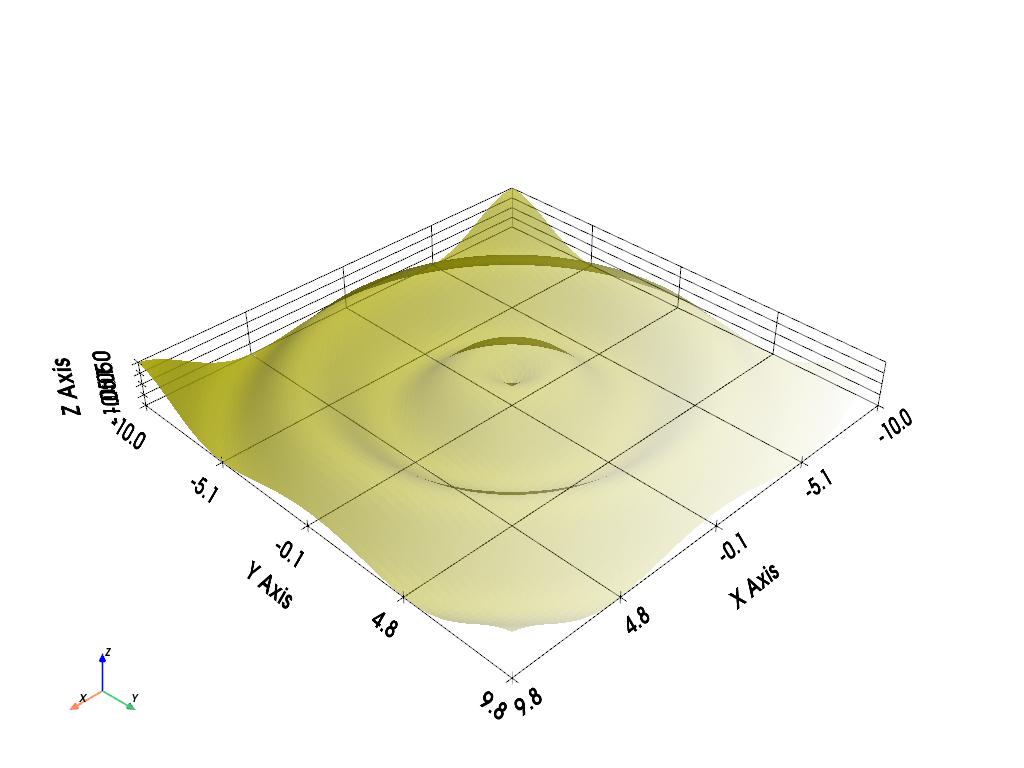
Textures with Transparency#
Textures can also specify per-pixel opacity values. The image must
contain a 4th channel specifying the opacity value from 0 [transparent] to
255 [fully visible]. To enable this feature just pass the opacity array as the
4th channel of the image as a 3 dimensional matrix with shape [nrows, ncols, 4]
pyvista.numpy_to_texture().
Here we can download an image that has an alpha channel:
rgba = examples.download_rgba_texture()
rgba.n_components
4
# Render it
curvsurf.plot(texture=rgba, show_grid=True)
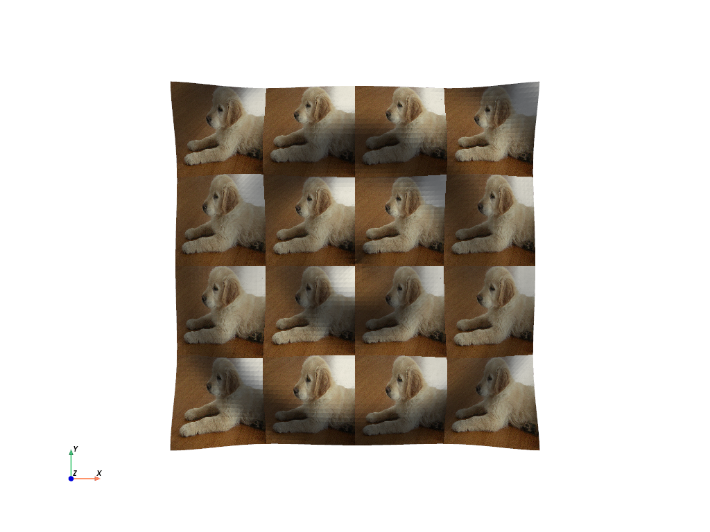
Repeating Textures#
What if you have a single texture that you’d like to repeat across a mesh? Simply define the texture coordinates for all nodes explicitly.
Here we create the texture coordinates to fill up the grid with several
mappings of a single texture. In order to do this we must define texture
coordinates outside of the typical (0, 1) range:
axial_num_puppies = 4
xc = np.linspace(0, axial_num_puppies, curvsurf.dimensions[0])
yc = np.linspace(0, axial_num_puppies, curvsurf.dimensions[1])

xxc, yyc = np.meshgrid(xc, yc)
puppy_coords = np.c_[yyc.ravel(), xxc.ravel()]
By defining texture coordinates that range (0, 4) on each axis, we will
produce 4 repetitions of the same texture on this mesh.
Then we must associate those texture coordinates with the mesh through the
pyvista.DataSet.active_texture_coordinates property.
Now display all the puppies.
# use the puppy image
tex = examples.download_puppy_texture()
curvsurf.plot(texture=tex, cpos='xy')
Spherical Texture Coordinates#
We have a built in convienance method for mapping textures to spherical coordinate systems much like the planar mapping demoed above.
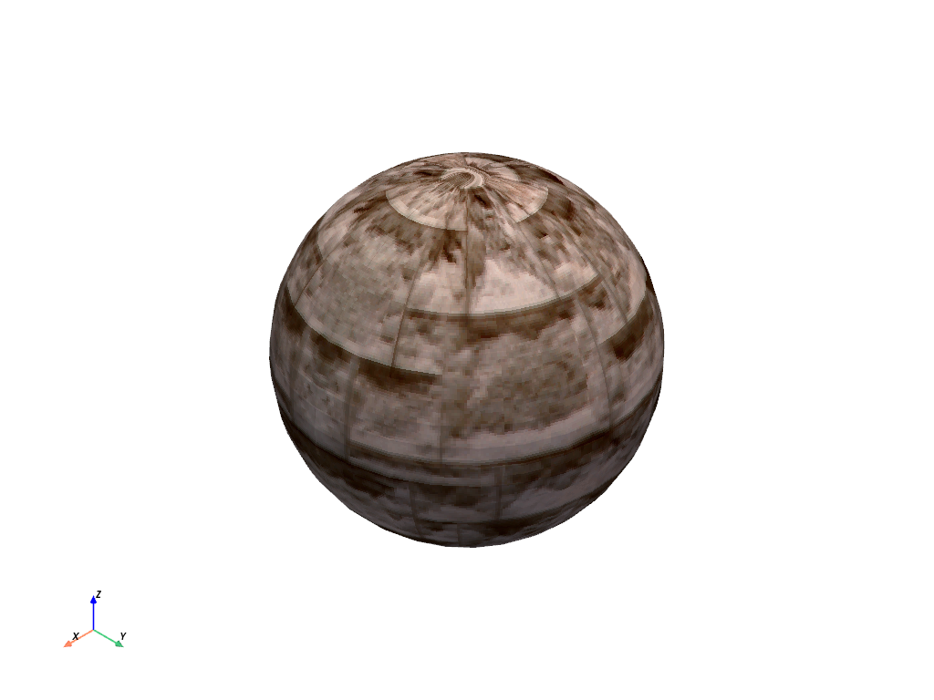
The helper method above does not always produce the desired texture coordinates, so sometimes it must be done manually. Here is a great, user contributed example from this support issue
Manually create the texture coordinates for a globe map. First, we create the mesh that will be used as the globe. Note the start_theta for a slight overlappig
sphere = pv.Sphere(
radius=1,
theta_resolution=120,
phi_resolution=120,
start_theta=270.001,
end_theta=270,
)
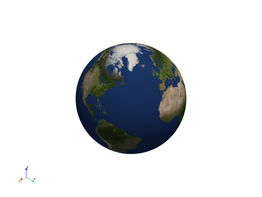
# Initialize the texture coordinates array
sphere.active_texture_coordinates = np.zeros((sphere.points.shape[0], 2))
# Populate by manually calculating
for i in range(sphere.points.shape[0]):
sphere.active_texture_coordinates[i] = [
0.5 + np.arctan2(-sphere.points[i, 0], sphere.points[i, 1]) / (2 * np.pi),
0.5 + np.arcsin(sphere.points[i, 2]) / np.pi,
]
# And let's display it with a world map
tex = examples.load_globe_texture()
sphere.plot(texture=tex)
Total running time of the script: (0 minutes 9.460 seconds)