Detailed Resampling

Download Python source code | Download Jupyter notebook

This example uses pyvista.DataObjectFilters.sample().

pyvista.DataObjectFilters.resample_to_image() samples onto a new ImageData in a single call.

pyvista.DataSetFilters.interpolate() is similar, and the two methods are compared in Compare Interpolation/Sampling Methods.

Resample one mesh’s point/cell arrays onto another mesh’s nodes.

This example will resample a volumetric mesh’s scalar data onto the surface of a sphere contained in that volume.

import pyvista as pv
from pyvista import examples

Simple Resample

Query a grid’s points onto a sphere

mesh = pv.Sphere(center=(4.5, 4.5, 4.5), radius=4.5)
data_to_probe = examples.load_uniform()

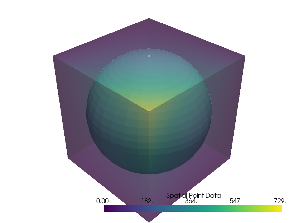
Plot the two datasets

pl = pv.Plotter()
pl.add_mesh(mesh, color=True)
pl.add_mesh(data_to_probe, opacity=0.5)
pl.show()

Static Scene

Interactive Scene

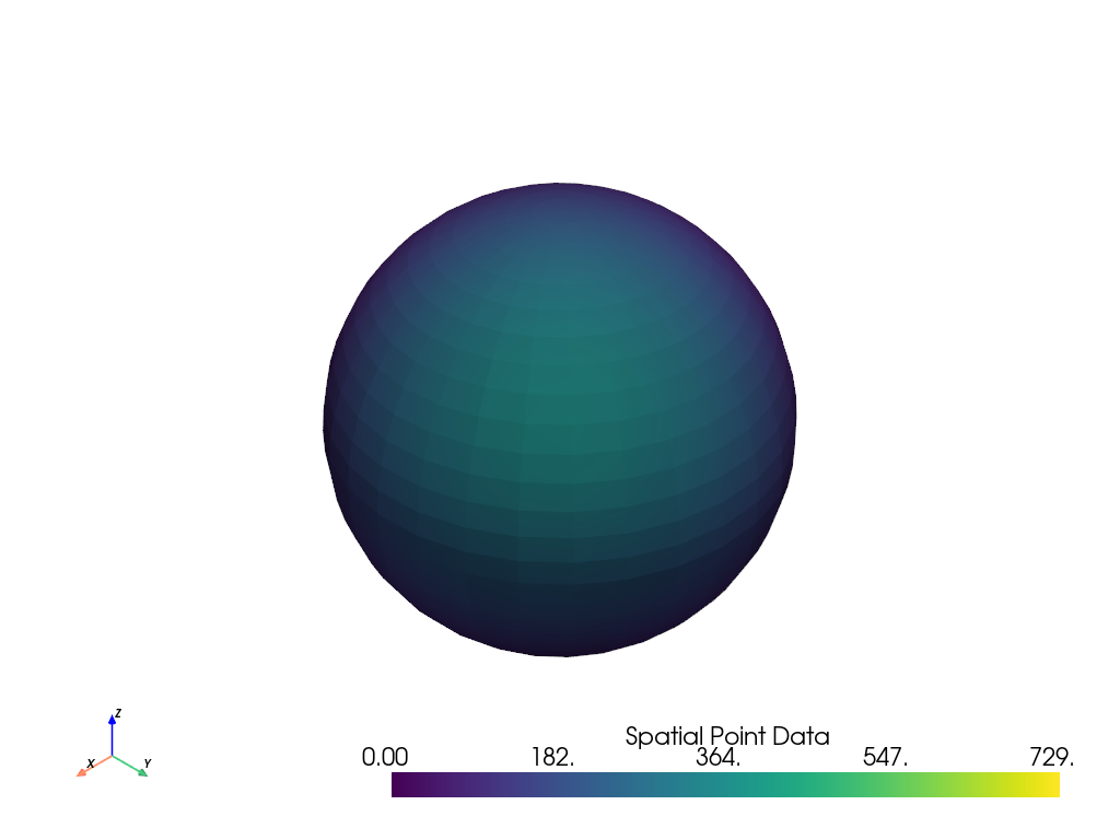
Run the algorithm and plot the result

result = mesh.sample(data_to_probe)

# Plot result
name = 'Spatial Point Data'
result.plot(scalars=name, clim=data_to_probe.get_data_range(name))

Static Scene

Interactive Scene

resample_to_image() samples onto a new ImageData instead. Pass a reference_volume to give the output the geometry of an image which already exists.

mesh.resample_to_image(reference_volume=data_to_probe)

ImageData (0x7f52f31d6d40)
  N Cells:      729
  N Points:     1000
  X Bounds:     0.000e+00, 9.000e+00
  Y Bounds:     0.000e+00, 9.000e+00
  Z Bounds:     0.000e+00, 9.000e+00
  Dimensions:   10, 10, 10
  Spacing:      1.000e+00, 1.000e+00, 1.000e+00
  N Arrays:     2

ImageData 1,000 points 729 cells 13 KiB

Bounds⧉X [0.000e+00, 9.000e+00]Y [0.000e+00, 9.000e+00]Z [0.000e+00, 9.000e+00]

Griddims 10 x 10 x 10spacing (1.000e+00, 1.000e+00, 1.000e+00)

• Point Data: (2)
  • Normals⧉
    3 comp
    float32
    [-9.860e-01, 9.860e-01]
    normals
  • vtkValidPointMask⧉
    scalar
    int8
    [0.000e+00, 1.000e+00]

Complex Resample

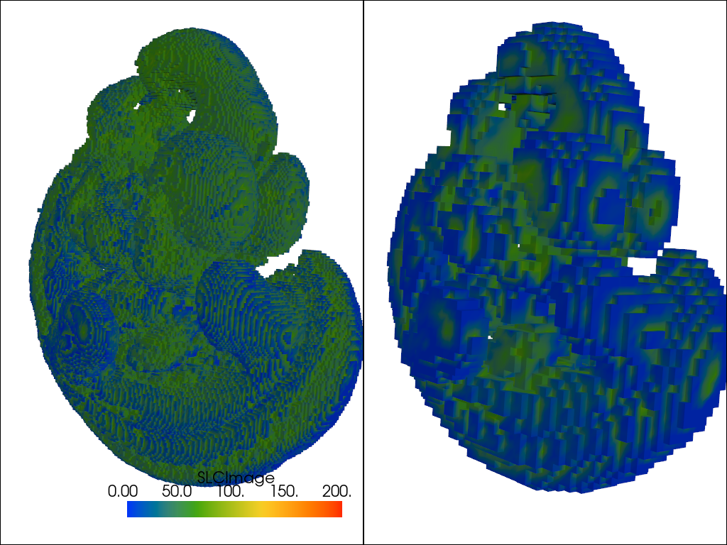
Take a volume of data and create a grid of lower resolution to resample on

data_to_probe = examples.download_embryo()
mesh = pv.create_grid(data_to_probe, dimensions=(75, 75, 75))

result = mesh.sample(data_to_probe)

resample_to_image() does both steps in one call.

data_to_probe.resample_to_image(dimensions=(75, 75, 75))

ImageData (0x7f52f31d46a0)
  N Cells:      405224
  N Points:     421875
  X Bounds:     1.700e+00, 2.533e+02
  Y Bounds:     1.700e+00, 2.533e+02
  Z Bounds:     1.700e+00, 2.533e+02
  Dimensions:   75, 75, 75
  Spacing:      3.400e+00, 3.400e+00, 3.400e+00
  N Arrays:     2

ImageData 421,875 points 405,224 cells 824 KiB

Bounds⧉X [1.700e+00, 2.533e+02]Y [1.700e+00, 2.533e+02]Z [1.700e+00, 2.533e+02]

Griddims 75 x 75 x 75spacing (3.400e+00, 3.400e+00, 3.400e+00)

• Point Data: (2)
  SLCImage active
  • SLCImage⧉
    scalar
    uint8
    [0.000e+00, 1.550e+02]
    active
  • vtkValidPointMask⧉
    scalar
    int8
    [1.000e+00, 1.000e+00]

To resample ImageData directly, use resample() instead.

data_to_probe.resample(dimensions=(75, 75, 75))

ImageData (0x7f52f31d4e20)
  N Cells:      405224
  N Points:     421875
  X Bounds:     1.207e+00, 2.538e+02
  Y Bounds:     1.207e+00, 2.538e+02
  Z Bounds:     1.207e+00, 2.538e+02
  Dimensions:   75, 75, 75
  Spacing:      3.413e+00, 3.413e+00, 3.413e+00
  N Arrays:     1

ImageData 421,875 points 405,224 cells 412 KiB

Bounds⧉X [1.207e+00, 2.538e+02]Y [1.207e+00, 2.538e+02]Z [1.207e+00, 2.538e+02]

Griddims 75 x 75 x 75spacing (3.413e+00, 3.413e+00, 3.413e+00)

• Point Data: (1)
  SLCImage active
  • SLCImage⧉
    scalar
    uint8
    [0.000e+00, 1.700e+02]
    active

threshold = lambda m: m.threshold(75.0, scalars='SLCImage')
cpos = pv.CameraPosition(
    position=(468.9, -152.8, 152.1),
    focal_point=(121.7, 140.3, 112.3),
    viewup=(-0.1088, 0.006229, 0.994),
)
dargs = dict(clim=[0, 200], cmap='rainbow')

pl = pv.Plotter(shape=(1, 2))
pl.add_mesh(threshold(data_to_probe), **dargs)
pl.subplot(0, 1)
pl.add_mesh(threshold(result), **dargs)
pl.link_views()
pl.view_isometric()
pl.show(cpos=cpos)

Static Scene

Interactive Scene

Resample a Processed Volume

Clipping an image returns an UnstructuredGrid, which image filters do not accept. resample_to_image() puts the processed volume back on a regular grid.

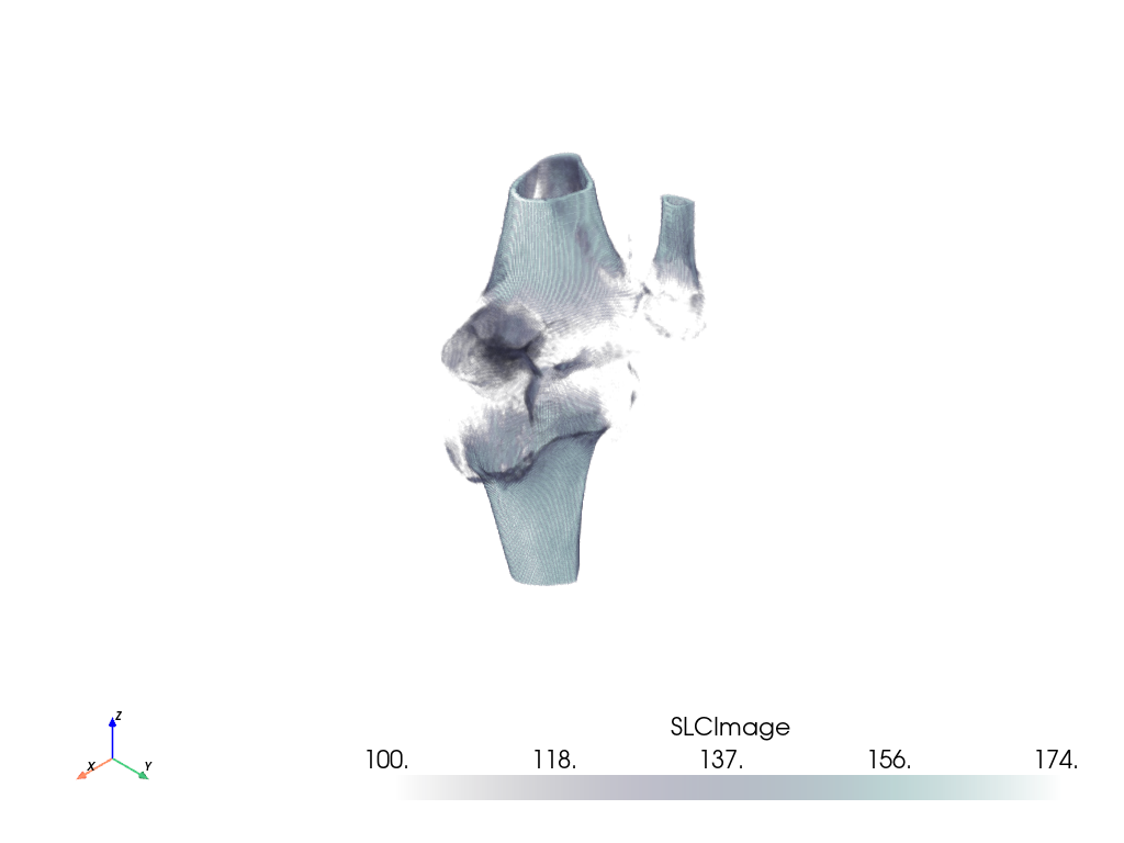
Start from a volumetric scan of a knee. Bone is the bright end of its intensity range, from 100 up.

knee = examples.download_knee_full()


knee.plot(volume=True, cmap='bone', clim=[100, 174])

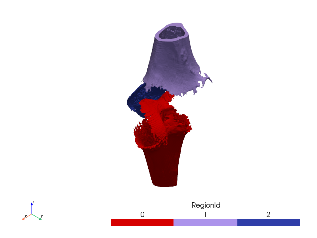
Clip the scan to the bone, and keep the three largest pieces: the tibia, the femur, and the patella. connectivity() numbers the regions from the largest down and stores the numbers as 'RegionId'.

bone = knee.clip_scalar(scalars='SLCImage', value=100, invert=False)
bones = bone.connectivity('specified', [0, 1, 2])
bones.plot(scalars='RegionId', cmap='glasbey', categories=True)

Static Scene

Interactive Scene

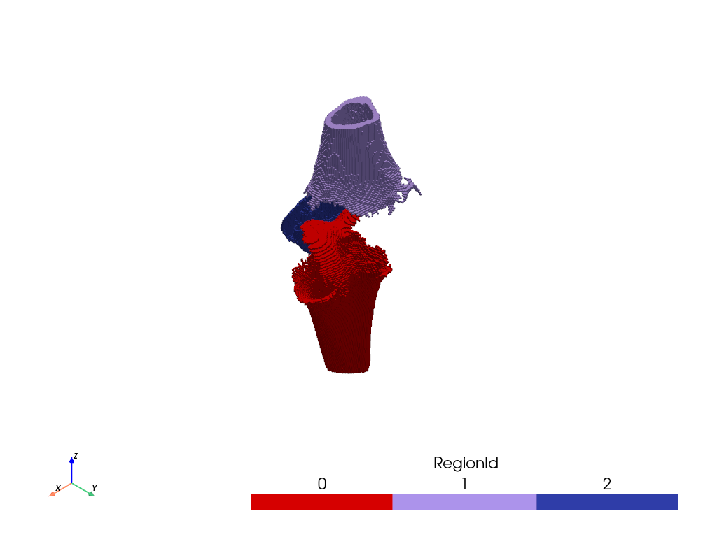
Resample the labeled bones onto the scan’s own grid with reference_volume, so that a voxel of the output is a voxel of the scan. Sample the labels as categories to keep them whole, and blank the voxels which fall outside the bone.

labels = bones.resample_to_image(reference_volume=knee, categorical=True, mark_blank=True)

The labels sit on the points of the image, so render them as voxel cells with points_to_cells().

labels.points_to_cells().plot(scalars='RegionId', cmap='glasbey', categories=True)

Static Scene

Interactive Scene

Tags: filter