ImageDataFilters.resample#
- ImageDataFilters.resample(
- sample_rate: float | VectorLikeFloat | None = None,
- interpolation: _InterpolationOptions = 'nearest',
- *,
- border_mode: _BorderModeOptions = 'clamp',
- reference_image: ImageData | None = None,
- dimensions: VectorLikeInt | None = None,
- spacing: float | VectorLikeFloat | None = None,
- rounding_func: Callable[[VectorLikeFloat], VectorLikeInt] | None = None,
- anti_aliasing: bool = False,
- premultiply_alpha: bool = False,
- is_srgb: bool = False,
- extend_border: bool | None = None,
- scalars: str | None = None,
- preference: PointLiteral | CellLiteral = 'point',
- inplace: bool = False,
- progress_bar: bool = False,
Resample the image to modify its dimensions and spacing.
The resampling can be controlled in several ways:
Specify the output geometry using a
reference_image.Specify the
dimensionsexplicitly.Specify the
sample_rateexplicitly.Specify the
spacingexplicitly.
Use
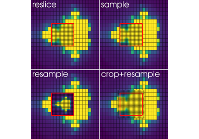
reference_imagefor full control of the resampled geometry. For all other options, the geometry is implicitly defined such that the resampled image fits the bounds of the input. In every case the image is resampled in its own frame; usereslice()to sample it at the points of another image instead.This filter may be used to resample either point or cell data. For point data, this filter assumes the data is from discrete samples in space which represent pixels or voxels; the resampled bounds are therefore extended by 1/2 voxel spacing by default though this may be disabled.
Note
Singleton input dimensions are not resampled by this filter, for example, 2D images will remain 2D. An output dimension may be reduced to a singleton, however, for example, to flatten a 3D volume into a single 2D slice.
Added in version 0.45.
Changed in version 0.49: Values are sampled at the centers of the resampled voxels when the border is extended and when resampling cell data. Previously the first and last samples were aligned with the first and last samples of the input, which offset the values from the points they are stored at by up to half the input spacing. Reducing an axis to a singleton now samples the center of that axis instead of its first slice.
- Parameters:
- sample_rate
float|VectorLikeFloat, optional Sampling rates to use. Can be a single value or vector of three values for each axis. Values greater than
1.0will up-sample the axis and values less than1.0will down-sample it. Values must be greater than0. The output dimensions are rounded to integers withrounding_func.Changed in version 0.50: Fractional dimensions are rounded with
numpy.round(). In version 0.49 they were rounded down.- interpolation‘nearest’, ‘linear’, ‘cubic’, ‘lanczos’, ‘hamming’, ‘blackman’, ‘bspline’
Interpolation mode to use.
'nearest'(default) duplicates (if up-sampling) or removes (if down-sampling) values but does not modify them.'linear'and'cubic'use linear and cubic interpolation, respectively.'lanczos','hamming', and'blackman'use a windowed sinc filter and may be used to preserve sharp details and/or reduce image artifacts.'bspline'uses an n-degree basis spline to smoothly interpolate across points. The default degree is3, but can range from0to9. Append the desired degree to the string to set it, for example,'bspline5'for a fifth-degree B-spline.
Added in version 0.47: Added
'bspline'interpolation.Note
use
'nearest'for pixel art or categorical data such as segmentation masksuse
'linear'for speed-critical tasksuse
'cubic'for upscaling or general-purpose resamplinguse
'lanczos'for high-detail down-sampling (at the cost of some ringing)use
'blackman'for minimizing ringing artifacts (at the cost of some detail)use
'hamming'for a balance between detail-preservation and reducing ringing
- border_mode‘clamp’ | ‘wrap’ | ‘mirror’, default: ‘clamp’
Controls the interpolation at the image’s borders.
'clamp'- values outside the image are clamped to the nearest edge.'wrap'- values outside the image are wrapped periodically along the axis.'mirror'- values outside the image are mirrored at the boundary.
Added in version 0.47.
- reference_image
ImageData, optional Reference image to use. If specified, the input is resized to the reference’s
dimensions, and the reference’sspacing,origin,offset, anddirection_matrixare applied to the output.Note
The image is resampled in its own frame and the reference’s geometry is applied to the result afterwards, so the values are not sampled at the reference image’s points. Use
reslice()to sample at those points.- dimensions
VectorLikeInt, optional Set the output
dimensionsof the resampled image.Note
Dimensions is the number of points along each axis. If resampling cell data, each dimension should be one more than the number of desired output cells (since there are
Ncells andN+1points along each axis). See examples.- spacing
float|VectorLikeFloat, optional Approximate
spacingof the resampled image. Can be a single value or vector of three values for each axis. Values must be greater than0. The output dimensions are rounded to integers withrounding_func, so the actual spacing may differ. The spacing divides the bounds of the image represented as cells, or the bounds of its points whenextend_borderisFalse. Singleton axes keep their spacing. See examples.Added in version 0.50.
- rounding_func
Callable[VectorLikeFloat,VectorLikeInt], optional Control how the dimensions computed from
spacingorsample_rateare rounded to integers. Should accept a length-3 vector containing the dimension values along the three directions and return a length-3 vector.numpy.round()is used by default.Rounding the dimensions implies rounding the actual spacing.
Cannot be set together with
reference_imageordimensions.Added in version 0.50.
- anti_aliasingbool, default:
False Enable anti-aliasing to reduce image artifacts when down-sampling. Each down-sampled axis is blurred in proportion to its sampling ratio before resampling, which approximates averaging the samples it merges. Has no effect on axes that are not down-sampled.
Changed in version 0.49: The blur is sized from each axis’s own sampling ratio. Previously a fixed blur was applied to all three axes, including axes which are not down-sampled, which left aliasing at large sampling ratios and blurred more than necessary at small ones.
- premultiply_alphabool, default:
False Treat the scalars as straight (unassociated) RGBA colors and weight the colors by alpha while resampling. The color channels are multiplied by alpha before interpolating and divided by the interpolated alpha afterwards, so the color of transparent pixels does not bleed into their neighbors. Each color channel is clipped to its range over the input pixels that are not fully transparent, alpha is clipped to its range over the input, and fully transparent output pixels have a color of
0. The scalars must have four components.Added in version 0.50.
- is_srgbbool, default:
False Treat the scalars as sRGB-encoded RGB or RGBA colors and resample them in linear light. The color channels are decoded to linear values before interpolating and encoded back to sRGB afterwards, so blending light and dark colors does not darken them. Alpha is not decoded. The scalars must have three or four components and be
uint8in the range[0, 255]or floating point in the range[0, 1]. Color channels are clipped to that range.Added in version 0.50.
- extend_borderbool, optional
Extend the apparent input border by approximately half the
spacing. If enabled, the bounds of the resampled points will be larger than the input image bounds. Enabling this option also has the effect that the re-sampled spacing will directly correlate with the resampled dimensions, for example, if the dimensions are doubled the spacing will be halved. The values are sampled at the centers of the resampled voxels. See examples.This option is enabled by default when resampling point data. Has no effect when resampling cell data or when a
reference_imageis provided.- scalars
str, optional Name of scalars to resample. Defaults to currently active scalars.
- preference
str, default: ‘point’ When scalars is specified, this is the preferred array type to search for in the dataset. Must be either
'point'or'cell'.- inplacebool, default:
False If
True, resample the image in-place. By default, a newImageDatainstance is returned.- progress_barbool, default:
False Display a progress bar to indicate progress.
- sample_rate
- Returns:
ImageDataResampled image.
Examples#
Download Python source code | Download Jupyter notebook
Create a small 2D grayscale image with dimensions 3 x 2 for demonstration.
>>> import pyvista as pv
>>> import numpy as np
>>> from pyvista import examples
>>> image = pv.ImageData(dimensions=(3, 2, 1))
>>> image.point_data['data'] = np.linspace(0, 255, 6, dtype=np.uint8)
Define a custom plotter to show the image. Although the image data is defined
as point data, we use points_to_cells() to display the image as
PIXEL (or VOXEL) cells
instead. Grayscale coloring is used and the camera is adjusted to fit the image.
>>> def image_plotter(image: pv.ImageData, clim=(0, 255)) -> pv.Plotter:
...     pl = pv.Plotter()
...     image = image.points_to_cells()
...     pl.add_mesh(
...         image,
...         lighting=False,
...         show_edges=True,
...         cmap='grey',
...         clim=clim,
...         show_scalar_bar=False,
...         line_width=3,
...     )
...     pl.view_xy()
...     pl.camera.tight()
...     pl.enable_anti_aliasing()
...     return pl
Show the image.
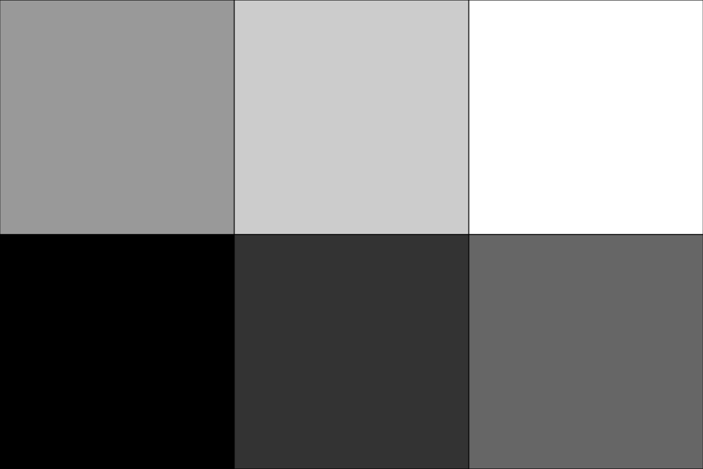
Use sample_rate to up-sample the image. 'nearest' interpolation is
used by default.
>>> upsampled = image.resample(sample_rate=2.0)
>>> plot = image_plotter(upsampled)
>>> plot.show()
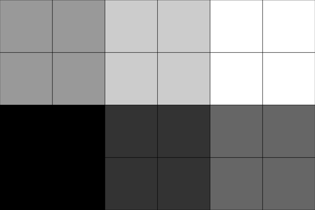
Use 'linear' interpolation. Note that the argument names sample_rate
and interpolation may be omitted.
>>> upsampled = image.resample(2.0, 'linear')
>>> plot = image_plotter(upsampled)
>>> plot.show()
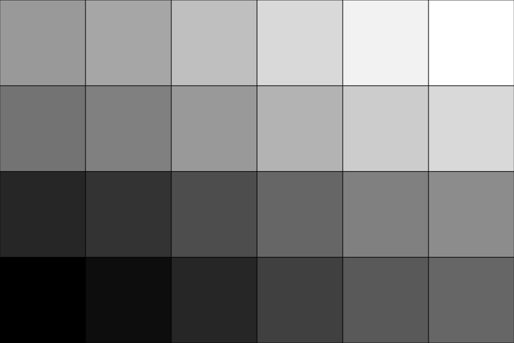
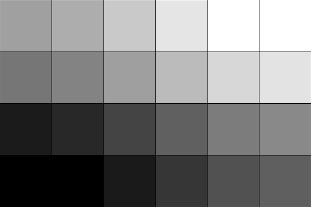
Use 'cubic' interpolation. Here we also specify the output
dimensions explicitly instead of using sample_rate.
>>> upsampled = image.resample(dimensions=(6, 4, 1), interpolation='cubic')
>>> plot = image_plotter(upsampled)
>>> plot.show()
Alternatively, specify the output spacing. The dimensions are rounded to
integers, so the actual spacing is only approximate.
>>> spaced = image.resample(spacing=(0.7, 0.4, 1.0))
>>> spaced.dimensions
(4, 5, 1)
>>> spaced.spacing
(0.75, 0.4, 1.0)
Use rounding_func=np.ceil to force the actual spacing to be no larger than
the requested spacing.
>>> spaced = image.resample(spacing=(0.7, 0.4, 1.0), rounding_func=np.ceil)
>>> spaced.dimensions
(5, 5, 1)
>>> spaced.spacing
(0.6, 0.4, 1.0)
Compare the relative physical size of the image before and after resampling.
>>> image
ImageData (...)
  N Cells:      2
  N Points:     6
  X Bounds:     0.000e+00, 2.000e+00
  Y Bounds:     0.000e+00, 1.000e+00
  Z Bounds:     0.000e+00, 0.000e+00
  Dimensions:   3, 2, 1
  Spacing:      1.000e+00, 1.000e+00, 1.000e+00
  N Arrays:     1
>>> upsampled
ImageData (...)
  N Cells:      15
  N Points:     24
  X Bounds:     -2.500e-01, 2.250e+00
  Y Bounds:     -2.500e-01, 1.250e+00
  Z Bounds:     0.000e+00, 0.000e+00
  Dimensions:   6, 4, 1
  Spacing:      5.000e-01, 5.000e-01, 1.000e+00
  N Arrays:     1
Note that the up-sampled dimensions are doubled and
the spacing is halved (as expected). Also note,
however, that the physical bounds of the input differ from the output.
The up-sampled origin also differs:
>>> image.origin
(0.0, 0.0, 0.0)
>>> upsampled.origin
(-0.25, -0.25, 0.0)
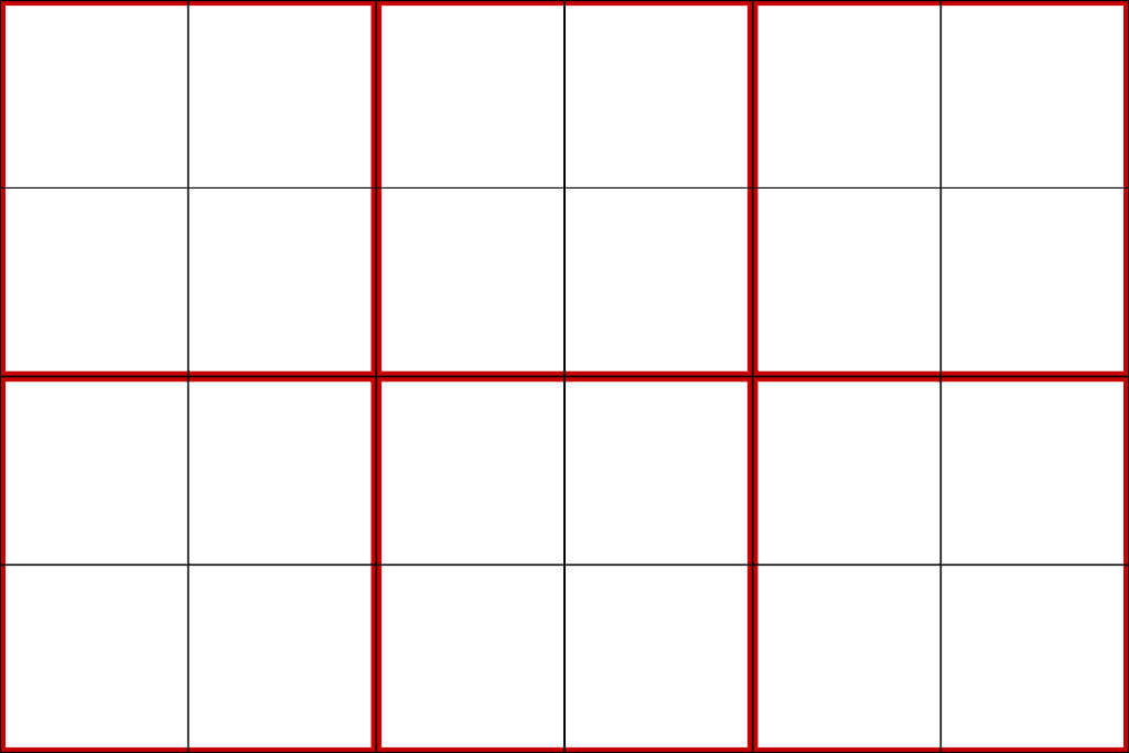
This is because the resampling is done with extend_border enabled by default
which adds a half cell-width border to the image and adjusts the origin and
spacing such that the bounds match when the image is represented as cells.
Apply points_to_cells() to the input and resampled images and show that
the bounds match.
>>> image_as_cells = image.points_to_cells()
>>> image_as_cells.bounds
BoundsTuple(x_min = -0.5,
            x_max =  2.5,
            y_min = -0.5,
            y_max =  1.5,
            z_min =  0.0,
            z_max =  0.0)
>>> upsampled_as_cells = upsampled.points_to_cells()
>>> upsampled_as_cells.bounds
BoundsTuple(x_min = -0.5,
            x_max =  2.5,
            y_min = -0.5,
            y_max =  1.5,
            z_min =  0.0,
            z_max =  0.0)
Plot the two images together as wireframe to visualize them. The original is in red, and the resampled image is in black.
>>> pl = pv.Plotter()
>>> _ = pl.add_mesh(
...     image_as_cells, style='wireframe', color='red', line_width=10
... )
>>> _ = pl.add_mesh(
...     upsampled_as_cells, style='wireframe', color='black', line_width=2
... )
>>> pl.view_xy()
>>> pl.camera.tight()
>>> pl.show()
Disable extend_border to force the input and output bounds of the points
to be the same instead.
>>> upsampled = image.resample(sample_rate=2, extend_border=False)
Compare the two images again.
>>> image
ImageData (...)
  N Cells:      2
  N Points:     6
  X Bounds:     0.000e+00, 2.000e+00
  Y Bounds:     0.000e+00, 1.000e+00
  Z Bounds:     0.000e+00, 0.000e+00
  Dimensions:   3, 2, 1
  Spacing:      1.000e+00, 1.000e+00, 1.000e+00
  N Arrays:     1
>>> upsampled
ImageData (...)
  N Cells:      15
  N Points:     24
  X Bounds:     0.000e+00, 2.000e+00
  Y Bounds:     0.000e+00, 1.000e+00
  Z Bounds:     0.000e+00, 0.000e+00
  Dimensions:   6, 4, 1
  Spacing:      4.000e-01, 3.333e-01, 1.000e+00
  N Arrays:     1
This time the input and output bounds match without any further processing. Like before, the dimensions have doubled; unlike before, however, the spacing is not halved, but is instead smaller than half which is necessary to ensure the bounds remain the same. Also unlike before, the origin is unaffected:
>>> image.origin
(0.0, 0.0, 0.0)
>>> upsampled.origin
(0.0, 0.0, 0.0)
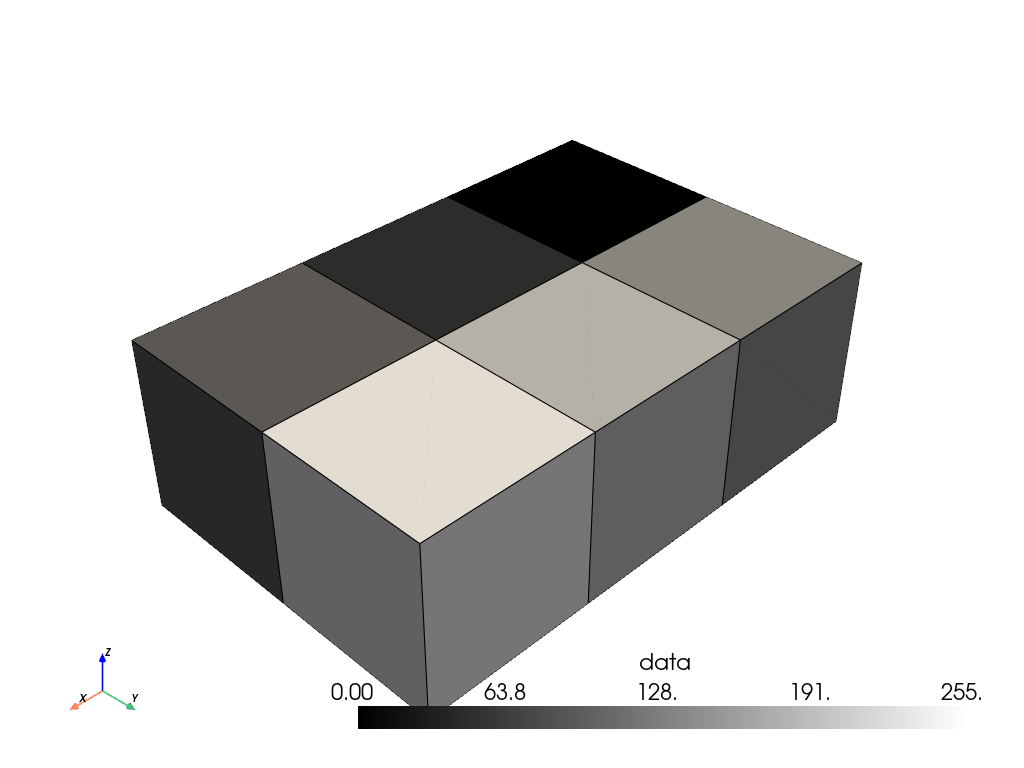
All the above examples are with 2D images with point data. However, the filter also works with 3D volumes and will also work with cell data.
Convert the 2D image with point data into a 3D volume with cell data and plot it for context.
>>> volume = image.points_to_cells(dimensionality='3D')
>>> volume.plot(show_edges=True, cmap='grey')
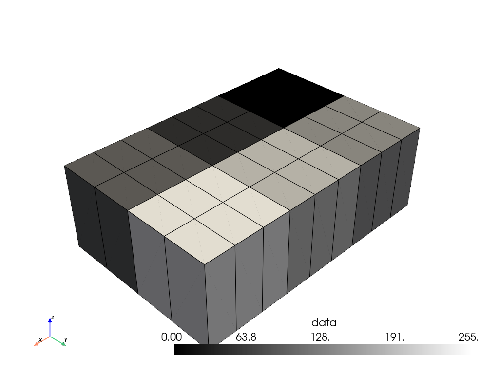
Up-sample the volume. Set the sampling rate for each axis separately.
>>> resampled = volume.resample(sample_rate=(3.0, 2.0, 1.0))
>>> resampled.plot(show_edges=True, cmap='grey')
Alternatively, we could have set the dimensions explicitly. Since we want
9 x 4 x 1 cells along the x-y-z axes (respectively), we set the dimensions
to (10, 5, 2), that is, one more than the desired number of cells.
>>> resampled = volume.resample(dimensions=(10, 5, 2))
>>> resampled.plot(show_edges=True, cmap='grey')
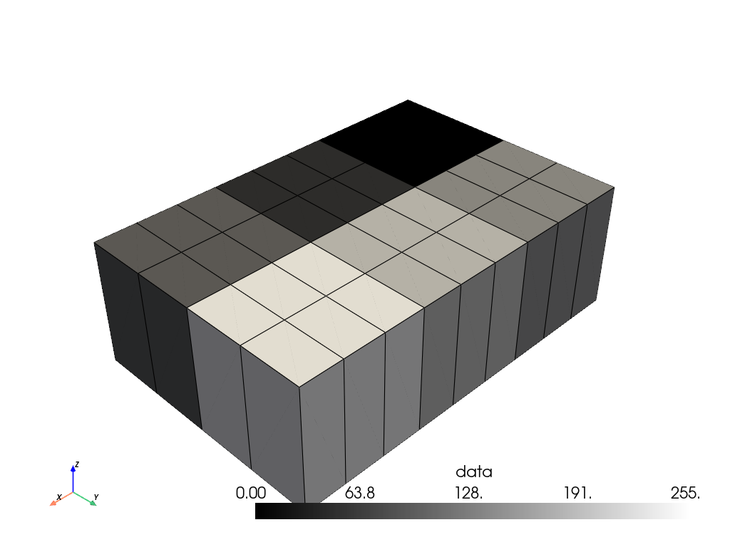
Compare the bounds before and after resampling. Unlike with point data, the bounds are not (and cannot be) extended.
>>> volume.bounds
BoundsTuple(x_min = -0.5,
            x_max =  2.5,
            y_min = -0.5,
            y_max =  1.5,
            z_min = -0.5,
            z_max =  0.5)
>>> resampled.bounds
BoundsTuple(x_min = -0.5,
            x_max =  2.5,
            y_min = -0.5,
            y_max =  1.5,
            z_min = -0.5,
            z_max =  0.5)
Use a reference image to control the resampling instead. Here we load two
images with different dimensions:
download_bird() and
download_gourds().
>>> bird = examples.download_bird()
>>> bird.dimensions
(458, 342, 1)
>>> gourds = examples.download_gourds()
>>> gourds.dimensions
(640, 480, 1)
Use reference_image to resample the bird to match the gourds geometry or
vice-versa.
>>> bird_resampled = bird.resample(reference_image=gourds)
>>> bird_resampled.dimensions
(640, 480, 1)
>>> gourds_resampled = gourds.resample(reference_image=bird)
>>> gourds_resampled.dimensions
(458, 342, 1)
Down-sample the gourds image to 1/10 its original resolution using 'lanczos'
interpolation.
>>> downsampled = gourds.resample(1 / 8, 'lanczos')
>>> downsampled.dimensions
(80, 60, 1)
Compare the downsampled image to the original and zoom in to show detail.
>>> kwargs = dict(
...     rgba=True,
...     lighting=False,
...     show_axes=False,
...     cpos='xy',
...     border_color='white',
...     border_width=6,
... )
>>> pv.plot_compare(
...     {'original': gourds, 'downsampled': downsampled}, zoom=3, **kwargs
... )
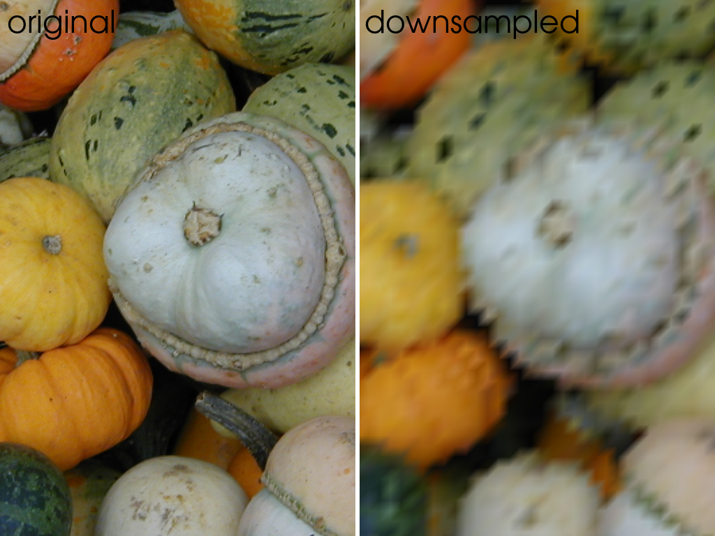
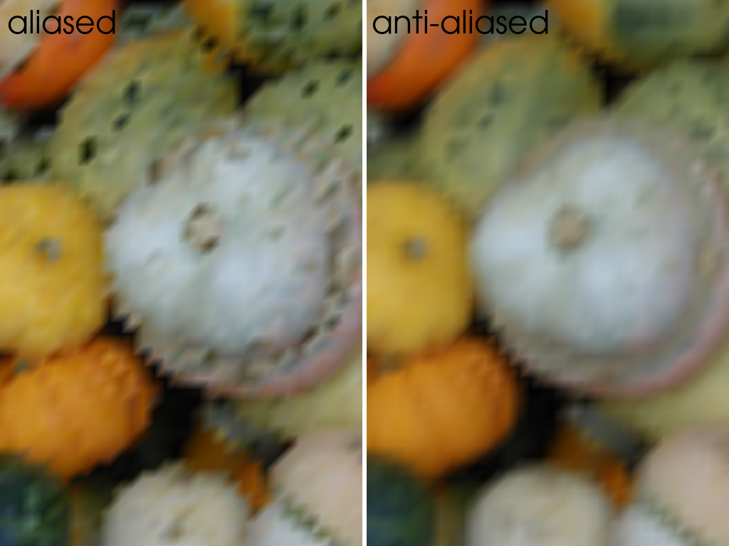
Note that down-sampling can create image artifacts caused by aliasing. Enable anti-aliasing to smooth the image before resampling.
>>> downsampled2 = gourds.resample(1 / 8, 'lanczos', anti_aliasing=True)
Compare down-sampling with and without anti-aliasing.
>>> pv.plot_compare(
...     {'aliased': downsampled, 'anti-aliased': downsampled2},
...     zoom=3,
...     **kwargs,
... )
Resample RGBA colors with transparency. Here two opaque red pixels are next to two fully transparent white pixels, like the background of a screenshot taken with a transparent background.
>>> rgba = pv.ImageData(dimensions=(4, 1, 1))
>>> rgba['rgba'] = np.array(
...     [[255, 0, 0, 255]] * 2 + [[255, 255, 255, 0]] * 2, dtype=np.uint8
... )
By default, the color and alpha channels are interpolated independently, so the white of the transparent pixels bleeds into the half-transparent pixel and turns it pink.
>>> rgba.resample(dimensions=(3, 1, 1), interpolation='linear')['rgba']
pyvista_ndarray([[255,   0,   0, 255],
                 [255, 128, 128, 128],
                 [255, 255, 255,   0]], dtype=uint8)
Enable premultiply_alpha to weight the colors by their alpha instead. The
half-transparent pixel stays red.
>>> rgba.resample(
...     dimensions=(3, 1, 1), interpolation='linear', premultiply_alpha=True
... )['rgba']
pyvista_ndarray([[255,   0,   0, 255],
                 [255,   0,   0, 128],
                 [  0,   0,   0,   0]], dtype=uint8)
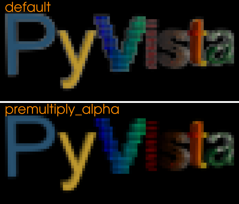
Down-sample the PyVista logo, which has a transparent background.
>>> logo = examples.load_logo()
>>> straight = logo.resample(1 / 16, 'lanczos', anti_aliasing=True)
>>> premultiplied = logo.resample(
...     1 / 16, 'lanczos', anti_aliasing=True, premultiply_alpha=True
... )
Show the images over black, as an image viewer would. Focus on the i and
s, which are partly transparent. By default, the white stored in the
transparent pixels bleeds into them and washes them out. With
premultiply_alpha, the i stays red and the s stays brown.
>>> def over_black(image):
...     rgba = image.active_scalars
...     image['rgb'] = (rgba[:, :3] * (rgba[:, 3:] / 255)).astype(np.uint8)
...     return image.points_to_cells(scalars='rgb')
>>> pv.plot_compare(
...     {
...         'default': over_black(straight),
...         'premultiply_alpha': over_black(premultiplied),
...     },
...     zoom=2.6,
...     window_size=[800, 682],
...     label_kwargs={'color': 'darkorange'},
...     shape=(2, 1),
...     **kwargs,
... )
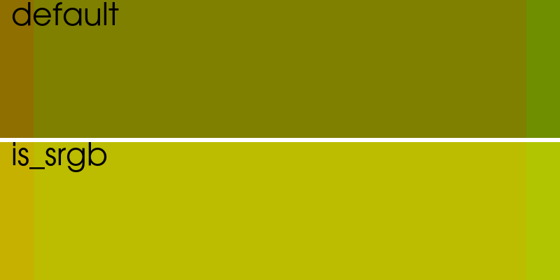
Colors are also blended in their sRGB encoding by default. Down-sample red and green stripes, which look yellow from a distance.
>>> stripes = pv.ImageData(dimensions=(32, 8, 1))
>>> red_green = np.array([[255, 0, 0], [0, 255, 0]], dtype=np.uint8)
>>> stripes['rgb'] = np.tile(red_green, (stripes.n_points // 2, 1))
>>> encoded = stripes.resample(0.5, 'linear', anti_aliasing=True)
Enable is_srgb to blend them in linear light instead. The default blends
the stripes to a dark olive, and is_srgb to yellow.
>>> linear = stripes.resample(0.5, 'linear', anti_aliasing=True, is_srgb=True)
>>> pv.plot_compare(
...     {
...         'default': encoded.points_to_cells(),
...         'is_srgb': linear.points_to_cells(),
...     },
...     zoom=4.2,
...     window_size=[800, 400],
...     label_kwargs={'color': 'black'},
...     shape=(2, 1),
...     **kwargs,
... )
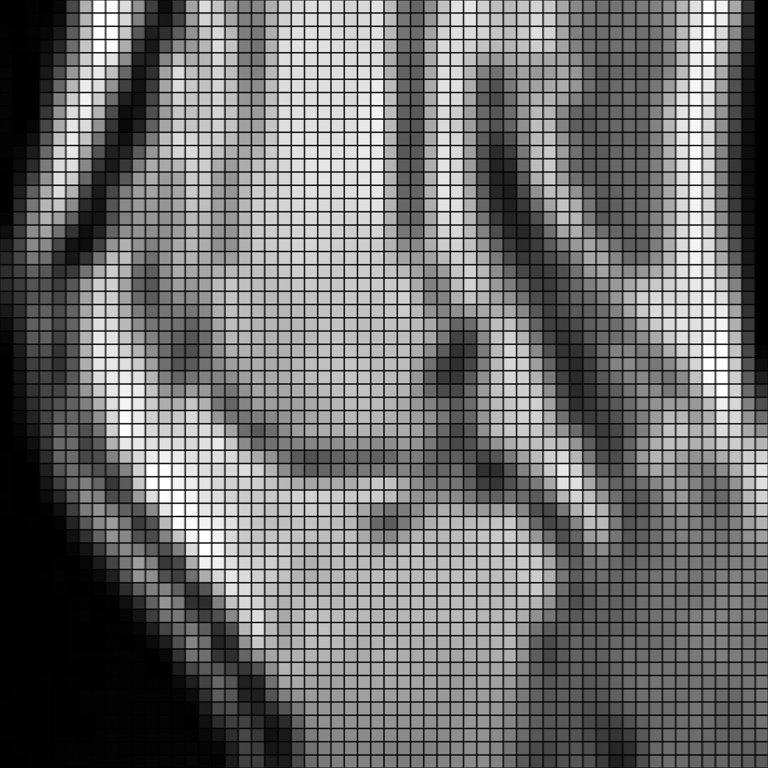
Load an MRI of a knee and down-sample it.
>>> knee = pv.examples.download_knee().resample(
...     0.1, 'linear', anti_aliasing=True
... )
Crop and plot it.
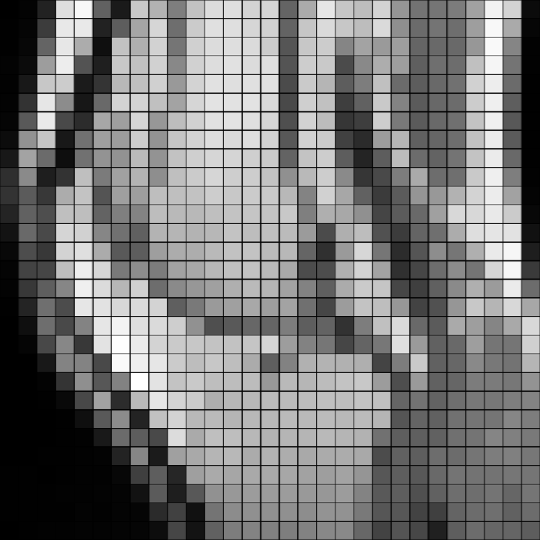
Up-sample it with B-spline interpolation. The interpolation is very smooth.
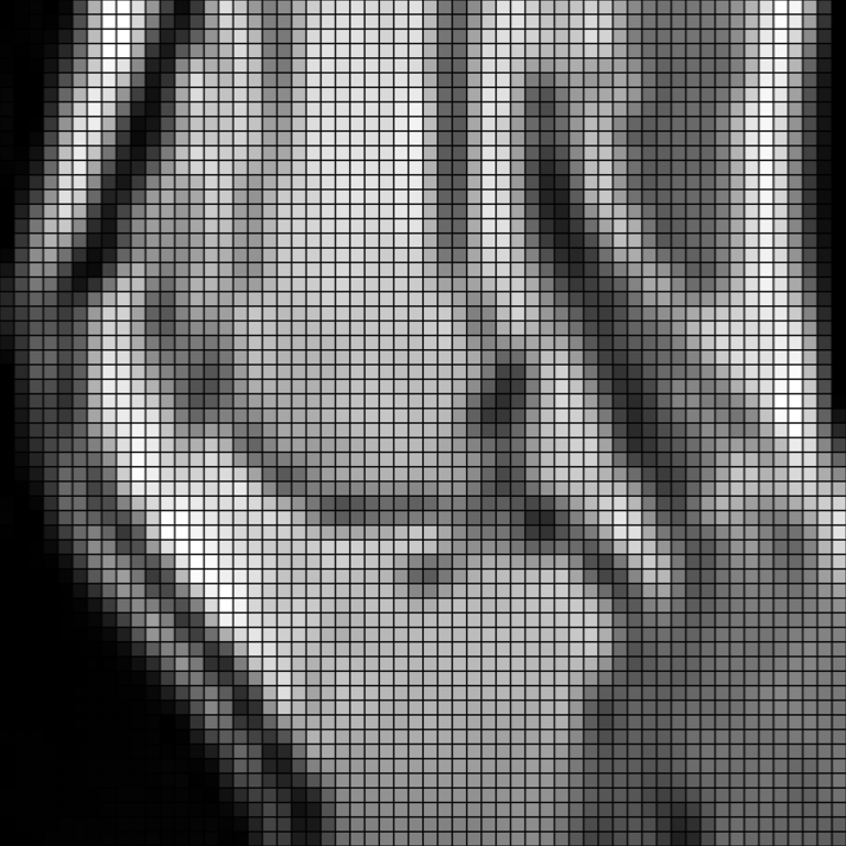
Use the 'wrap' border mode. Note how points at the border are brighter than previously,
since the bright pixels from the opposite edge are now included in the interpolation.
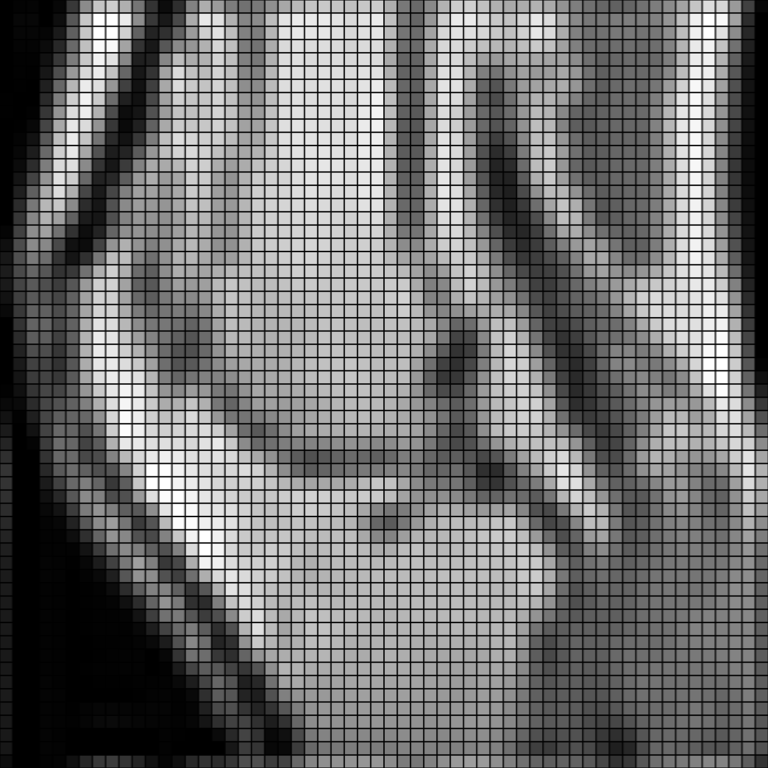
Compare B-spline interpolation to 'hamming'.
See Also#
resliceSample an image at the points of a reference image.
cropCrop image to remove points at the image’s boundaries.
sample()Resample array data from one mesh onto another.
resample_to_image()Resample a mesh of any type onto a new image.
interpolate()Interpolate values from one mesh onto another.
- Image Data Representations
Compare images represented as points vs. cells.
Used In#
API Examples
download_damavand_volcano(1 use)
Gallery Examples