Volume Rendering#
Download Python source code | Download Jupyter notebook
Volume render uniform mesh types like pyvista.ImageData or 3D NumPy arrays.
This also explores how to extract a volume of interest (VOI) from a
pyvista.ImageData using the
pyvista.ImageDataFilters.extract_subset() filter.
import numpy as np
import pyvista as pv
from pyvista import examples


# Download a volumetric dataset
vol = examples.download_knee_full()
vol
Simple Volume Render#
# A nice camera position
cpos = pv.CameraPosition(
    position=(-381.7, -46.02, 216.5),
    focal_point=(74.83, 89.29, 100.0),
    viewup=(0.23, 0.072, 0.97),
)

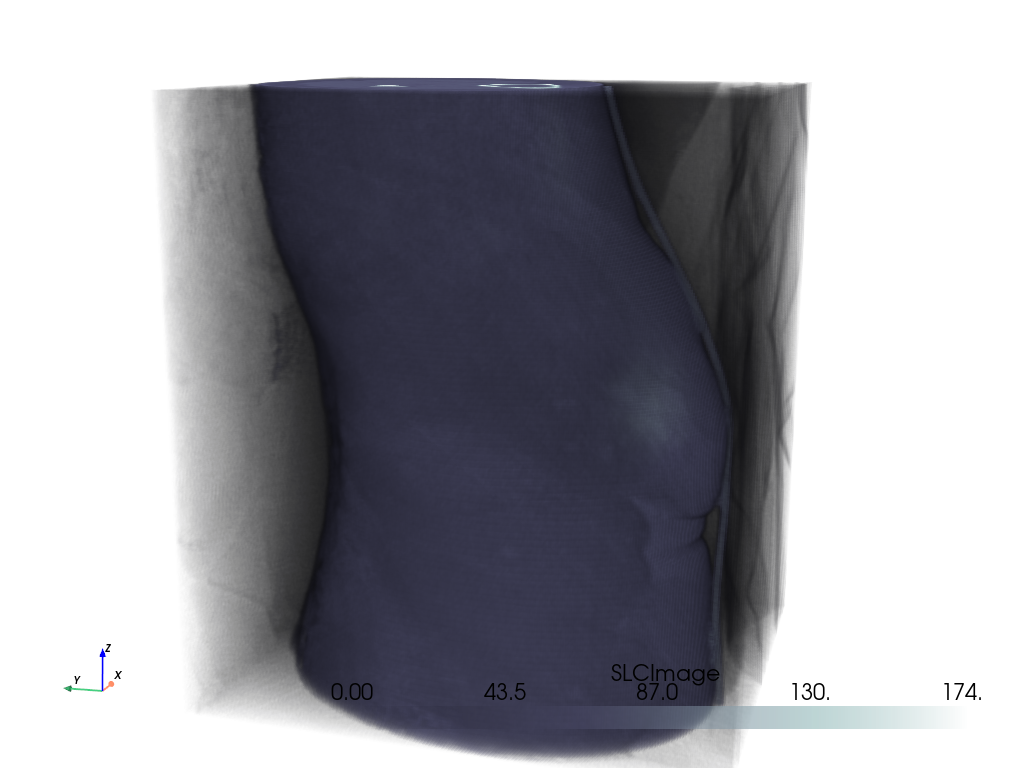
vol.plot(volume=True, cmap='bone', cpos=cpos)
Opacity Mappings#
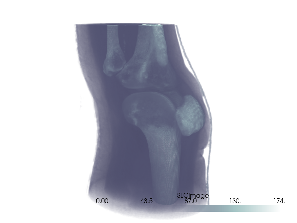
Or use the pyvista.Plotter.add_volume() method like below.
Note that here we use a non-default opacity mapping to a sigmoid:
pl = pv.Plotter()
pl.add_volume(vol, cmap='bone', opacity='sigmoid')
pl.camera_position = cpos
pl.show()
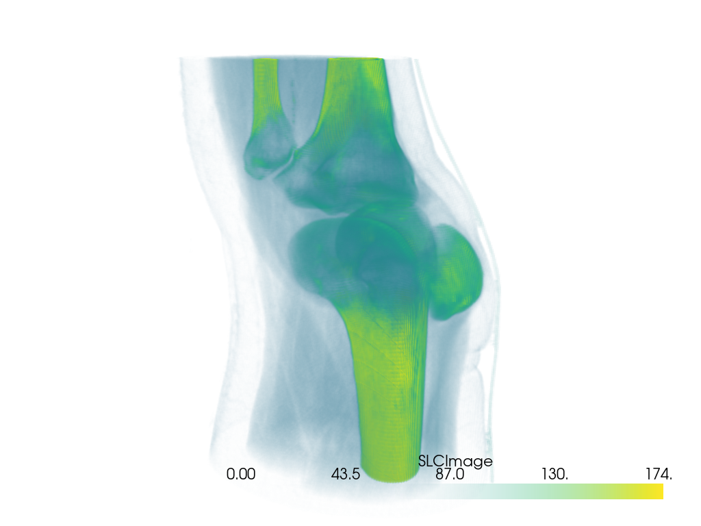
You can also use a custom opacity mapping
opacity = [0, 0, 0, 0.1, 0.3, 0.6, 1]

pl = pv.Plotter()
pl.add_volume(vol, cmap='viridis', opacity=opacity)
pl.camera_position = cpos
pl.show()
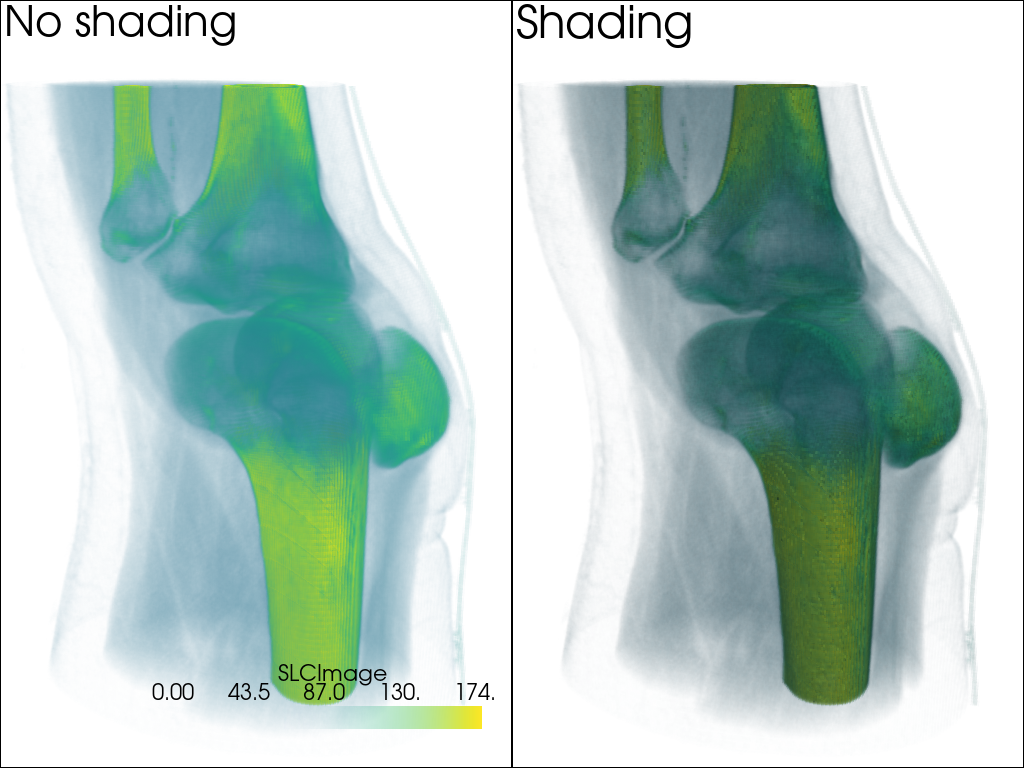
We can also use a shading technique when volume rendering with the shade
option
pl = pv.Plotter(shape=(1, 2))
pl.add_volume(vol, cmap='viridis', opacity=opacity, shade=False)
pl.add_text('No shading')
pl.camera_position = cpos
pl.subplot(0, 1)
pl.add_volume(vol, cmap='viridis', opacity=opacity, shade=True)
pl.add_text('Shading')
pl.link_views()
pl.show()
Cool Volume Examples#
Here are a few more cool volume rendering examples.
Head Dataset#
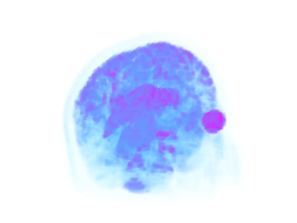
head = examples.download_head()

pl = pv.Plotter()
pl.add_volume(head, cmap='cool', opacity='sigmoid_6', show_scalar_bar=False)
pl.camera_position = pv.CameraPosition(
    position=(-228.0, -418.0, -158.0),
    focal_point=(94.0, 122.0, 82.0),
    viewup=(-0.2, -0.3, 0.9),
)
pl.camera.zoom(1.5)
pl.show()
Bolt-Nut MultiBlock Dataset#
Note
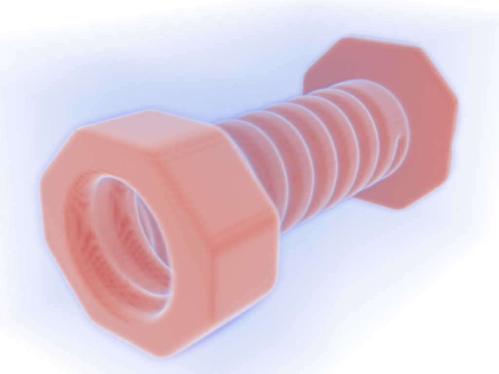
See how we set interpolation to 'linear' here to smooth out scalars of
each individual cell to make a more appealing plot. Two actor are returned
by add_volume because bolt_nut is a pyvista.MultiBlock
dataset.
bolt_nut = examples.download_bolt_nut()

pl = pv.Plotter()
actors = pl.add_volume(
    bolt_nut, cmap='coolwarm', opacity='sigmoid_5', show_scalar_bar=False
)
actors[0].prop.interpolation_type = 'linear'
actors[1].prop.interpolation_type = 'linear'
pl.camera_position = pv.CameraPosition(
    position=(127.4, -68.3, 88.2),
    focal_point=(30.3, 54.3, 26.0),
    viewup=(-0.25, 0.28, 0.93),
)
cpos = pl.show(return_cpos=True)
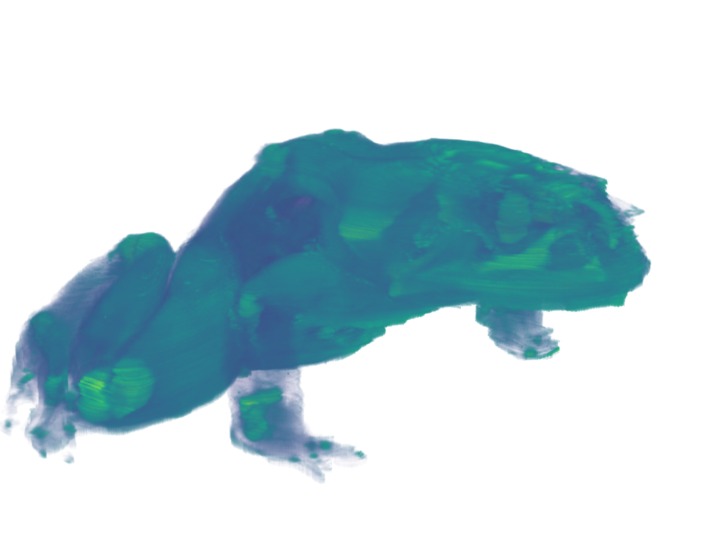
Frog Dataset#
frog = examples.download_frog()

pl = pv.Plotter()
pl.add_volume(frog, cmap='viridis', opacity='sigmoid_6', show_scalar_bar=False)
pl.camera_position = pv.CameraPosition(
    position=(929.0, 1067.0, -278.9),
    focal_point=(249.5, 234.5, 101.2),
    viewup=(-0.2048, -0.2632, -0.9427),
)
pl.camera.zoom(1.5)
pl.show()
Extracting a VOI#
Use the pyvista.ImageDataFilters.extract_subset() filter to extract
a volume of interest/subset volume to volume render. This is ideal when
dealing with particularly large volumes and you want to volume render only
a specific region.
# Load a particularly large volume
large_vol = examples.download_damavand_volcano()
large_vol
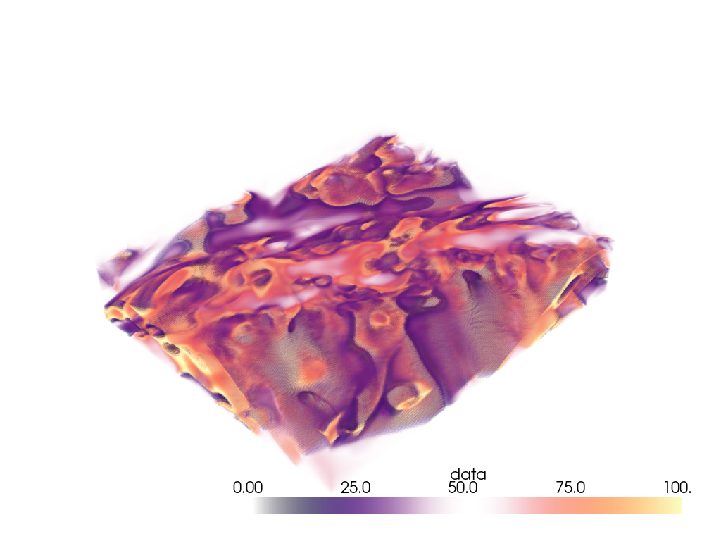
Whoa, that’s a big volume. We probably don’t want to volume render the whole thing. So let’s extract a region of interest under the volcano.
The region we will extract will be between nodes 175 and 200 on the x-axis, between nodes 105 and 132 on the y-axis, and between nodes 98 and 170 on the z-axis.
voi = large_vol.extract_subset([175, 200, 105, 132, 98, 170])

pl = pv.Plotter()
pl.add_mesh(large_vol.outline(), color='k')
pl.add_mesh(voi, cmap='magma')
pl.show()
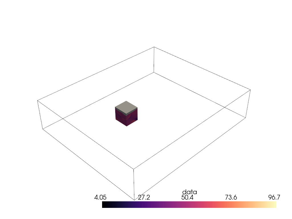
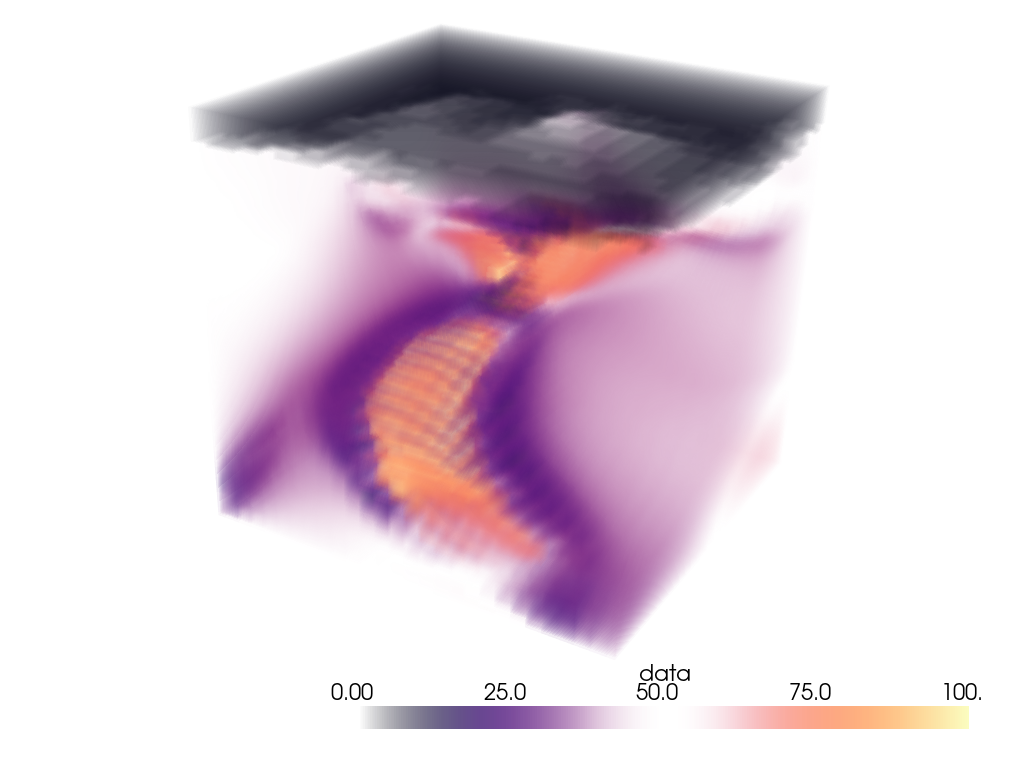
Ah, much better. Let’s now volume render that region of interest.
pl = pv.Plotter()
pl.add_volume(voi, cmap='magma', clim=clim, opacity=opacity, opacity_unit_distance=2000)
pl.camera_position = pv.CameraPosition(
    position=(531600.0, 3944000.0, 26560.0),
    focal_point=(599100.0, 3982000.0, -11970.0),
    viewup=(0.3739, 0.2443, 0.8947),
)
pl.show()
Volume With Segmentation Mask#
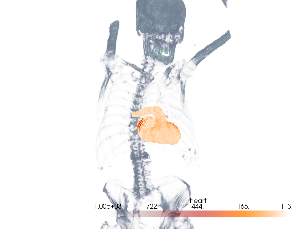
Visualize a medical image with a corresponding binary segmentation mask.
For this example, we use download_whole_body_ct_male()
though download_whole_body_ct_female(), or any
other dataset with a corresponding label or mask may be used.
Load the dataset and get the ct image and a mask image. Here, a mask of the heart is used.
dataset = examples.download_whole_body_ct_male()
ct_image = dataset['ct']
heart_mask = dataset['segmentations']['heart']
Use the segmentation mask to isolate the heart in the CT image.
Initialize a new array and image with CT background values. Here, we set the scalar
values to -1000 which typically corresponds to air (low density).
heart_array = np.full_like(ct_image.active_scalars, -1000)
Extract the intensities for the heart segment. We use heart mask’s array to mask the CT image to only extract the intensities of interest.
Add the masked array to the CT image as a new set of scalar values.
ct_image['heart'] = heart_array
Create the plot.
For the CT image, the opacity is set to a sigmoid function to show the
subject’s skeleton. Since different images have different intensity
distributions, you may need to experiment with different sigmoid functions.
See add_volume() for details.
pl = pv.Plotter()

# Add the CT image.
pl.add_volume(
    ct_image,
    scalars='NIFTI',
    cmap='bone',
    opacity='sigmoid_15',
    show_scalar_bar=False,
)

# Add masked CT image of the heart and use a contrasting color map.
_ = pl.add_volume(
    ct_image,
    scalars='heart',
    cmap='gist_heat',
    opacity='linear',
    opacity_unit_distance=np.mean(ct_image.spacing),
)

# Orient the camera to provide a latero-anterior view.
pl.view_yz()
pl.camera.azimuth = 70
pl.camera.up = (0, 0, 1)
pl.camera.zoom(1.5)
pl.show()
Total running time of the script: (0 minutes 13.625 seconds)