StructuredSphere

StructuredSphere(

*,

radius: float | VectorLike[float] = 0.5,

center: VectorLike[float] = (0.0, 0.0, 0.0),

direction: VectorLike[float] = (0.0, 0.0, 1.0),

theta_resolution: int = 30,

phi_resolution: int = 30,

start_theta: float = 0.0,

end_theta: float = 360.0,

start_phi: float = 0.0,

end_phi: float = 180.0,

) → StructuredGrid

Create a sphere as a StructuredGrid.

The grid is generated in spherical coordinates and has an i-j-k ordering where i, j, and k correspond to the radial, polar (phi), and azimuthal (theta) directions, respectively. Like CylinderStructured(), a single radius generates a 2D surface of QUAD cells whereas a sequence of radii generates a 3D volume of HEXAHEDRON cells.

PyVista uses a convention where theta represents the azimuthal angle (similar to degrees longitude on the globe) and phi represents the polar angle (similar to degrees latitude on the globe). In contrast to latitude on the globe, here phi is 0 degrees at the North Pole and 180 degrees at the South Pole. phi=0 is on the positive z-axis by default. theta=0 is on the positive x-axis by default.

With a sequence of radii the tessellation matches SolidSphere() at the same resolutions, cell for cell and by volume; only the storage differs. Every cell here is a HEXAHEDRON, collapsed to a wedge shape at the poles where SolidSphere() uses WEDGE cells and no coincident points, and only SolidSphere() can fill the center. Prefer this function for the i-j-k ordering, which addresses the grid by radius, phi and theta directly.

Note that the poles have degenerate cells with coincident points, and that a full 360-degree sweep of theta has a seam of duplicate points where the start and end angles meet. Both are required by the grid’s structure. Use Sphere() with tessellation='phi_theta' for a 2D surface, or SolidSphere() for a 3D volume; neither has coincident points or degenerate cells.

Added in version 0.49.

Parameters:

radiusfloat | sequence[float], default: 0.5

Sphere radius, which must be greater than zero. If a sequence, then describes the radial coordinates of the cells as a range of values, and generates a 3D grid with concentric layers of cells. The sequence must be sorted in strictly ascending order.

centersequence[float], default: (0.0, 0.0, 0.0)

Center coordinate vector in [x, y, z].

directionsequence[float], default: (0.0, 0.0, 1.0)

Direction coordinate vector in [x, y, z] pointing from center to the sphere’s North Pole at zero degrees phi.

theta_resolutionint, default: 30

Set the number of points in the azimuthal direction (ranging from start_theta to end_theta).

Note

The k dimension of the structured grid is always one more than this value. For a full 360-degree sweep the extra point is the duplicate closing the seam.

phi_resolutionint, default: 30

Set the number of points in the polar direction (ranging from start_phi to end_phi).

start_thetafloat, default: 0.0

Starting azimuthal angle in degrees.

end_thetafloat, default: 360.0

Ending azimuthal angle in degrees. Must be greater than start_theta and within 360 degrees of it.

start_phifloat, default: 0.0

Starting polar angle in degrees [0, 180].

end_phifloat, default: 180.0

Ending polar angle in degrees [0, 180]. Must be greater than start_phi.

Returns:

pyvista.StructuredGrid

Structured sphere.

Examples

Download Python source code | Download Jupyter notebook

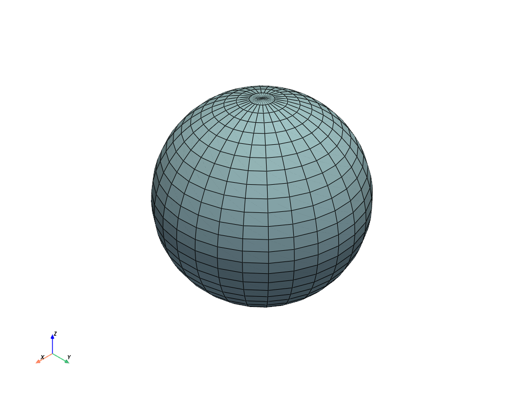
Create a sphere as a structured surface using default parameters.

>>> import numpy as np
>>> import pyvista as pv
>>> sphere = pv.StructuredSphere()
>>> sphere.plot(show_edges=True)

Static Scene

Interactive Scene

The dimensions follow the i-j-k ordering: one entry per radius, then phi_resolution, then theta_resolution plus one.

>>> pv.StructuredSphere(theta_resolution=20, phi_resolution=10).dimensions
(1, 10, 21)

Swapping the two resolutions swaps the last two dimensions, and the extra point stays with theta.

>>> pv.StructuredSphere(theta_resolution=10, phi_resolution=20).dimensions
(1, 20, 11)

Use a sequence of radii to set the first dimension and generate a 3D grid with concentric layers of cells. This is useful for modeling volumetric data such as an atmosphere.

>>> pv.StructuredSphere(
...     radius=[1.0, 1.5, 2.0], theta_resolution=20, phi_resolution=10
... ).dimensions
(3, 10, 21)

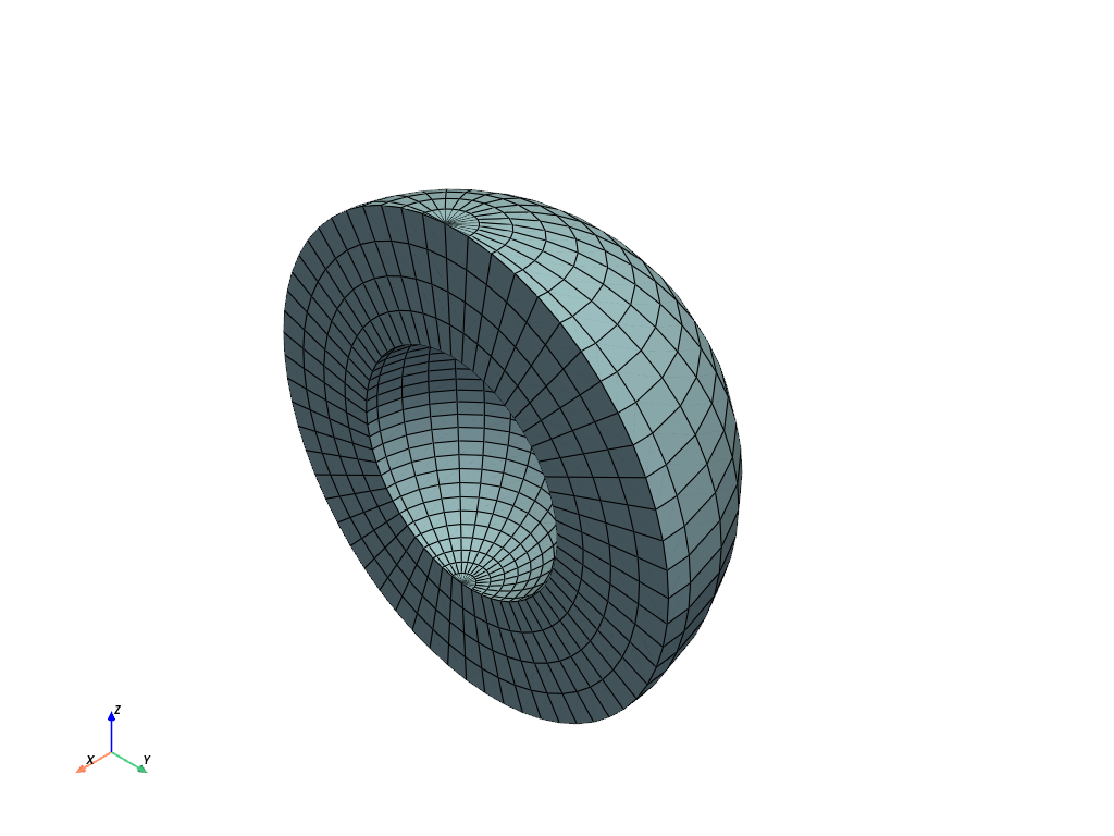
Show the layers by clipping the grid in half.

>>> sphere = pv.StructuredSphere(radius=np.linspace(1, 2, 5))
>>> sphere.clip(normal='x').plot(show_edges=True)

Static Scene

Interactive Scene

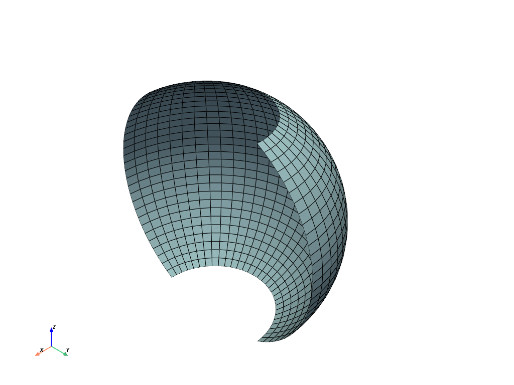
Create a partial sphere by restricting the angular ranges.

>>> sphere = pv.StructuredSphere(
...     start_theta=90, end_theta=270, start_phi=30, end_phi=150
... )
>>> sphere.plot(show_edges=True)

Static Scene

Interactive Scene

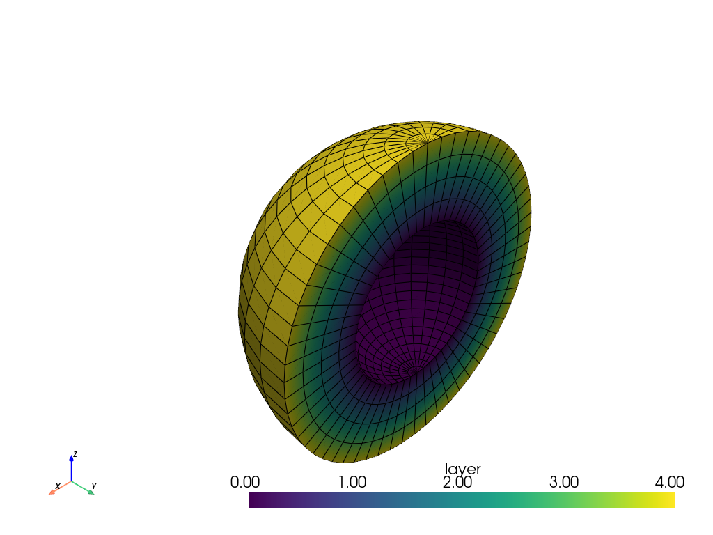
Use the i-j-k ordering to work with the grid by index. Since i is the radial axis, an array shaped like dimensions assigns a value per layer.

>>> sphere = pv.StructuredSphere(radius=np.linspace(1, 2, 5))
>>> layer = np.zeros(sphere.dimensions)
>>> layer[:] = np.arange(5).reshape(5, 1, 1)
>>> sphere['layer'] = layer.ravel(order='F')
>>> sphere.clip(normal='y').plot(scalars='layer', show_edges=True)

Static Scene

Interactive Scene

The same indexing selects part of the grid, here the outermost layer of points.

>>> outer = sphere.extract_subset([4, 4, 0, 29, 0, 30])
>>> outer.dimensions
(1, 30, 31)

See Also

pyvista.Sphere

Sphere that describes outer 2D surface.

pyvista.SolidSphere

Sphere that fills 3D space.

pyvista.SolidSphereGeneric

Solid sphere using flexible sampling.

pyvista.CylinderStructured

Cylinder as a StructuredGrid.

Used In

Gallery Examples

Create Sphere Mesh Multiple Ways

Create Sphere Mesh Multiple Ways

2 uses