Slicing Oblique Anatomy

Slicing Oblique Anatomy#

Download Python source code | Download Jupyter notebook

Put a scan on a structure’s own axes and slice it there.

A structure which runs across the scan axes is awkward to read in the slices the scanner produced. reslice() puts the scan on a grid aligned to the structure, and slice_orthogonal() and slice_index() then cut it squarely.

See Slicing for the slicing filters on an axis-aligned volume, and Reslice Images for what reslice does on its own.

import numpy as np

import pyvista as pv
from pyvista import examples

Find the Bone’s Axis#

Load a whole-body CT with its segmentations and take the left scapula, which lies at an angle within the axial plane.

dataset = examples.download_whole_body_ct_male()
ct = dataset['ct']
scapula = dataset['segmentations']['scapula_left']

The mask is drawn over the scan throughout, so give it an opacity array now: 0.3 on the bone and 0 everywhere else, which leaves the background transparent.

overlay = scapula.copy()
overlay['scapula'] = (scapula.active_scalars > 0) * 0.3
overlay.set_active_scalars('scapula')

(<FieldAssociation.POINT: 0>, pyvista_ndarray([0., 0., 0., ..., 0., 0., 0.], shape=(6988800,)))

Project the foreground of the bone’s mask onto the axial plane and fit a line to it there. Seeding init_direction pins the sign, so the fitted direction cannot come back reversed.

foreground = scapula.points[scapula.active_scalars > 0]
center = foreground.mean(axis=0)

in_plane = foreground.copy()
in_plane[:, 2] = center[2]
line, _, direction = pv.fit_line_to_points(in_plane, init_direction='x', return_meta=True)

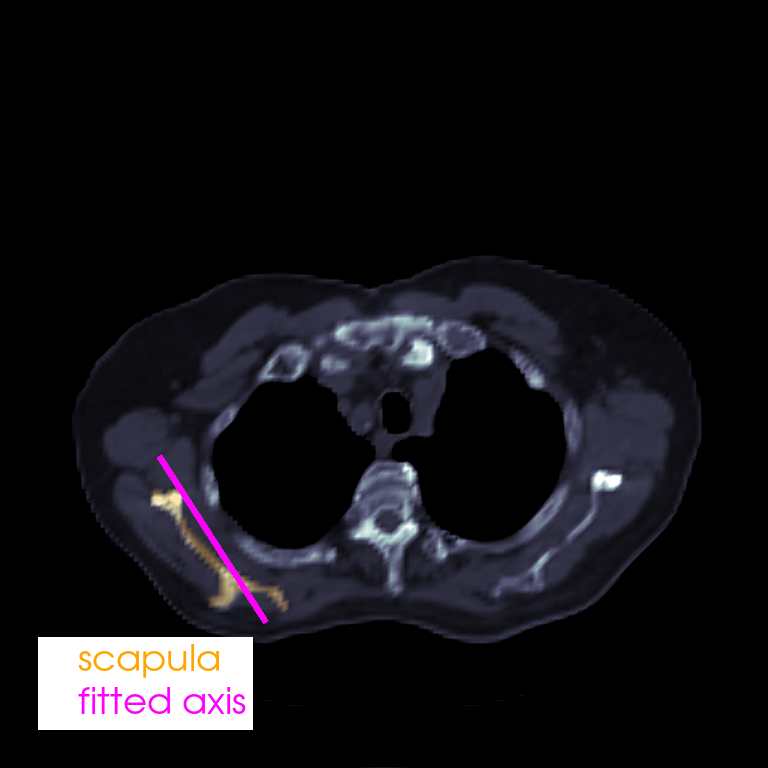
Draw the line over the axial slice it was fitted in. It crosses the slice at an angle, and so does the bone underneath it. The mask and the line are translated along +z to lift them clear of the image plane, which they would otherwise fight for depth.

index = round((center[2] - ct.origin[2]) / ct.spacing[2])
axial = ct.slice_index(k=index)
axial_mask = overlay.slice_index(k=index)


pl = pv.Plotter()
pl.add_mesh(axial, cmap='bone', clim=[-200, 900], show_scalar_bar=False, lighting=False)
pl.add_mesh(
    axial_mask.translate((0, 0, 0.5)),
    color='orange',
    opacity='scapula',
    lighting=False,
)
pl.add_mesh(line.translate((0, 0, 1)), color='magenta', line_width=6)
pl.add_legend(
    [['scapula', 'orange'], ['fitted axis', 'magenta']],
    bcolor='w',
    loc='lower left',
    size=(0.28, 0.12),
    face='none',
)
pl.view_xy()
pl.camera.tight()
pl.show()

Reslice Onto That Axis#

Because the fit is confined to that plane, a single rotation about the scan axis is enough to bring the line onto the image’s x axis.

angle = np.degrees(np.arctan2(direction[1], direction[0]))

plane = pv.ImageData(dimensions=(320, 220, 1), spacing=(1.0, 1.0, 1.0))


def placed(grid, rotation=0.0):
    """Return the transform which puts the scapula at the center of ``grid``."""
    return pv.Transform().translate(-center).rotate_z(rotation).translate(grid.center)

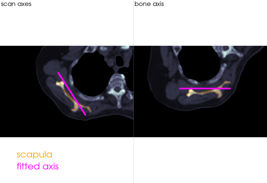
Reslice twice from that one grid, once without a rotation and once with it, and put the line and the bone’s mask through the same transforms so they can be compared against. The mask is a label image, so it takes 'nearest'.

along_scan = ct.reslice(plane, 'linear', transform=placed(plane), background_value=-1000)
along_bone = ct.reslice(
    plane, 'linear', transform=placed(plane, -angle), background_value=-1000
)

line_scan = line.transform(placed(plane), inplace=False)
line_bone = line.transform(placed(plane, -angle), inplace=False)

mask_scan = overlay.reslice(plane, 'nearest', transform=placed(plane), background_value=0)
mask_bone = overlay.reslice(
    plane, 'nearest', transform=placed(plane, -angle), background_value=0
)

The rotated grid samples along the bone. The bone itself comes out level, and so does the line it was fitted to.

pl = pv.Plotter(shape=(1, 2))
panels = [
    (along_scan, mask_scan, line_scan, 'scan axes'),
    (along_bone, mask_bone, line_bone, 'bone axis'),
]
for index, (image, mask, axis, label) in enumerate(panels):
    pl.subplot(0, index)
    pl.add_mesh(
        image,
        cmap='bone',
        clim=[-200, 900],
        show_scalar_bar=False,
        lighting=False,
    )
    pl.add_mesh(
        mask.translate((0, 0, 0.5)),
        color='orange',
        opacity='scapula',
        lighting=False,
    )
    pl.add_mesh(axis.translate((0, 0, 1)), color='magenta', line_width=6)
    pl.add_text(label, font_size=10)
    pl.view_xy()
    pl.camera.tight()
pl.subplot(0, 0)
pl.add_legend(
    [['scapula', 'orange'], ['fitted axis', 'magenta']],
    bcolor='w',
    loc='lower left',
    size=(0.4, 0.14),
    face='none',
)
pl.show()

Slice the Aligned Block#

The same rotation applied to a volume rather than a single plane gives a bone-aligned block of the scan. Reslice a generous one, then trim it to the bone with crop(), which works in index space and so needs the reslice to have happened first. See Crop Labeled ImageData for that filter on its own.

volume = pv.ImageData(dimensions=(200, 160, 280), spacing=(1.0, 1.0, 1.0))
block = ct.reslice(
    volume, 'linear', transform=placed(volume, -angle), background_value=-1000
)
bone = overlay.reslice(
    volume, 'nearest', transform=placed(volume, -angle), background_value=0
)

block = block.crop(mask=bone, padding=10)
bone = bone.crop(extent=block.extent)

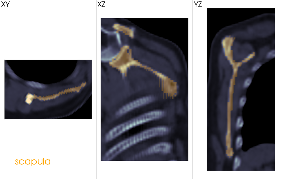
The trimmed block is axis-aligned, so slice_orthogonal() cuts the bone squarely along all three planes.

slices = block.slice_orthogonal()
mask_slices = bone.slice_orthogonal()

View each plane face-on. XZ shows the blade with its spine and the glenoid, and XY is a cross-section through it. None of these planes cut the bone this way in the axes the scanner produced.

pl = pv.Plotter(shape=(1, 3), window_size=[1000, 620])
for index, name in enumerate(['XY', 'XZ', 'YZ']):
    pl.subplot(0, index)
    pl.add_mesh(
        slices[name],
        cmap='bone',
        clim=[-200, 900],
        show_scalar_bar=False,
        lighting=False,
    )
    pl.add_mesh(mask_slices[name], color='orange', opacity='scapula', lighting=False)
    pl.add_text(name, font_size=10)
    pl.camera.tight(view=name.lower(), adjust_render_window=False, padding=0.1)
pl.subplot(0, 0)
pl.add_legend(
    [['scapula', 'orange']],
    bcolor='w',
    loc='lower left',
    size=(0.5, 0.09),
    face='none',
)
pl.show()

Choose the Slice Index#

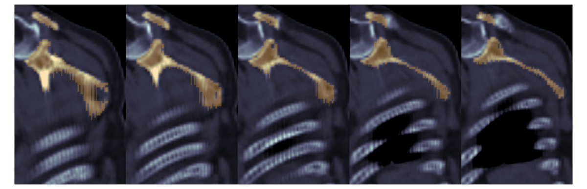
slice_orthogonal cuts at the block’s center. To cut elsewhere, use slice_index(), which takes an index along each axis and returns ImageData. Take five planes, stepping either side of the center index, and lay them side by side with concatenate().

step = 3
middle = block.dimensions[1] // 2
indices = [middle + count * step for count in range(-2, 3)]
planes = [block.slice_index(j=index) for index in indices]
masks = [bone.slice_index(j=index) for index in indices]

strip = planes[0].concatenate(planes[1:], 'x')
strip_mask = masks[0].concatenate(masks[1:], 'x')

The blade thins as the planes step back through it. The middle panel is the plane slice_orthogonal cut.

pl = pv.Plotter(window_size=[1200, 420])
pl.add_mesh(strip, cmap='bone', clim=[-200, 900], show_scalar_bar=False, lighting=False)
pl.add_mesh(strip_mask, color='orange', opacity='scapula', lighting=False)
pl.camera.tight(view='xz', padding=0.05)
pl.show()