Plot CFD Data

Plot a CFD example from OpenFoam hosted on the public SimScale examples at SimScale Project Library.

This example dataset was read using the pyvista.POpenFOAMReader. See Plot OpenFOAM data for a full example using this reader.

import numpy as np

import pyvista as pv
from pyvista import examples

Download and load the example dataset.

block = examples.download_openfoam_tubes()
block

Information	Blocks
MultiBlock Values N Blocks 2 X Bounds -0.128, 0.128 Y Bounds -0.028, 0.028 Z Bounds -0.014, 0.249	Index Name Type 0 internalMesh UnstructuredGrid 1 boundary MultiBlock

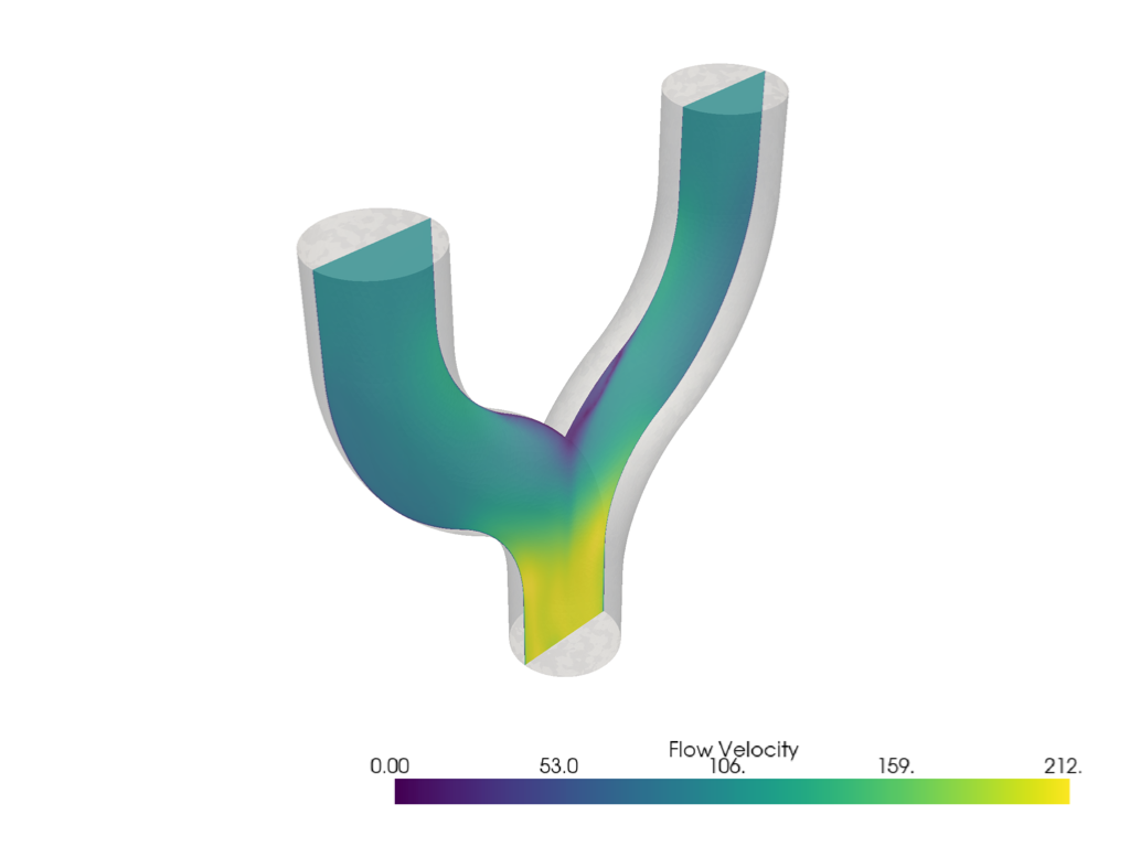
Plot Cross Section

Plot the outline of the dataset along with a cross section of the flow velocity.

# first, get the first block representing the air within the tube.
air = block[0]

# generate a slice in the XZ plane
y_slice = air.slice('y')

pl = pv.Plotter()
pl.add_mesh(y_slice, scalars='U', lighting=False, scalar_bar_args={'title': 'Flow Velocity'})
pl.add_mesh(air, color='w', opacity=0.25)
pl.enable_anti_aliasing()
pl.show()

Static Scene

Interactive Scene

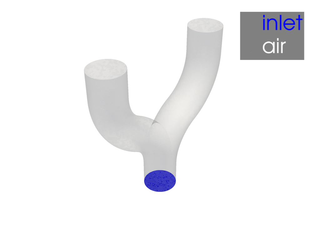
Plot Streamlines - Flow Velocity

Generate streamlines using streamlines_from_source().

# Let's use the inlet as a source. First plot it.
inlet = block[1][2]
pl = pv.Plotter()
pl.add_mesh(inlet, color='b', label='inlet')
pl.add_mesh(air, opacity=0.2, color='w', label='air')
pl.enable_anti_aliasing()
pl.add_legend(face=None)
pl.show()

Static Scene

Interactive Scene

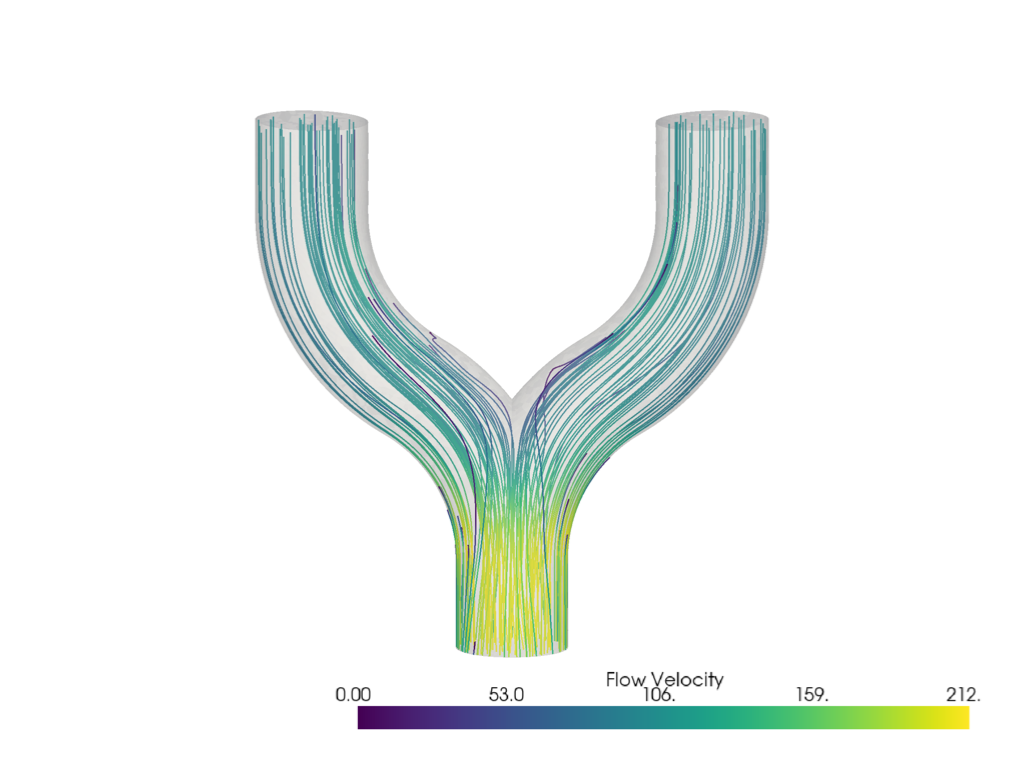
Now, actually generate the streamlines. Since the original inlet contains 1000 points, let’s reduce this to around 200 points by using every 5th point.

Note

If we wanted a uniform subsampling of the inlet, we could use pyvista/pyacvd

pset = pv.PointSet(inlet.points[::5])
lines = air.streamlines_from_source(
    pset,
    vectors='U',
    max_time=1.0,
)

pl = pv.Plotter()
pl.add_mesh(
    lines,
    render_lines_as_tubes=True,
    line_width=3,
    lighting=False,
    scalar_bar_args={'title': 'Flow Velocity'},
    scalars='U',
    rng=(0, 212),
)
pl.add_mesh(air, color='w', opacity=0.25)
pl.enable_anti_aliasing()
pl.camera_position = 'xz'
pl.show()

Static Scene

Interactive Scene

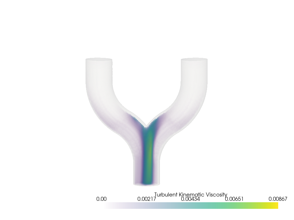
Volumetric Plot - Visualize Turbulent Kinematic Viscosity

The turbulent kinematic viscosity of a fluid is a derived quantity used in turbulence modeling to describe the effect of turbulent motion on the momentum transport within the fluid.

For this example, we will first sample the results from the pyvista.UnstructuredGrid onto a pyvista.ImageData using sample(). This is so we can visualize it using add_volume()

bounds = np.array(air.bounds) * 1.2
origin = (bounds[0], bounds[2], bounds[4])
spacing = (0.003, 0.003, 0.003)
dimensions = (
    int((bounds[1] - bounds[0]) // spacing[0] + 2),
    int((bounds[3] - bounds[2]) // spacing[1] + 2),
    int((bounds[5] - bounds[4]) // spacing[2] + 2),
)
grid = pv.ImageData(dimensions=dimensions, spacing=spacing, origin=origin)
grid = grid.sample(air)

pl = pv.Plotter()
vol = pl.add_volume(
    grid,
    scalars='nut',
    opacity='linear',
    scalar_bar_args={'title': 'Turbulent Kinematic Viscosity'},
)
vol.prop.interpolation_type = 'linear'
pl.add_mesh(air, color='w', opacity=0.1)
pl.camera_position = 'xz'
pl.show()